PHYSICS OF LEVITATION
Dimitri S. H. Charrier
Dimitri
Charrier / 2019 / http://dscharrier.free.fr
Intelligenti pauca
‘Few words suffice for he who understands’
Anonymous author
‘[relativity
theories] are made for believers: a believer will never oppose his guru’
Demetris
Christopoulos (researchgate.net)
Edition 2019
When I first got
interested to explore models and make experiments of innovative thrusters I
expected in the end that it could trigger passionate reactions. It is a healthy
reaction. Beginning at my individual level, the secondary effect was the
appropriation of this topic by other people. It means that the transfer of the
passion, message and idea is a success, in other words the message I wanted to
express has been received and well appreciated. I experienced it mainly after
the publication of articles.
While writing this
essay ‘Physics of Levitation’, I felt it was an interesting exercise. Maybe
because this domain is a little child of Physics. Personally when I grow up in
my education and instruction at school and university, I wish I could have had
in my hands such essay - even if it is really a personal vision - gathering
concepts and manners to levitate a solid object above the ground, such easy
thinking experiment, still today submitted to technological limits. Indeed, in
the literature such essays or books blending common levitating means with still
hypothetical ones are scarce, for not saying nonexistent. It has at least to be
read once for getting a reminder and a view on how basic effects, laws and
principles of physics can be turned into a beautiful scientific tool. A high potential
of technological applications and therefore benefits is possible.
However most of
all, I consider chapter 3 ‘Thermodynamic approach’ as a revolution. Indeed, it
reminds that the coupling of different physics can give birth to new visions
and opportunities. It is clearly not an engineering book. Do not hope to be
capable to build immediately a machine to levitate after having read this essay.
It is more an outsider than a well conventional, standard essay or book,
although its frame is strictly using academic and recognized notions of
physics.
Dimitri
Charrier
If you read these lines, it means
you are animated by a natural curiosity about levitation, which is the key
preliminary to innovative propulsions. This edition gathers notes and concepts
which I have written and collected since 2002. Future editions might come with
more examples of levitations, including advanced models. So far, this edition contains
demonstrations based on rigorous and classical physics. Still, the difficulty
was to give an apparent coherence in the construction of this topic, especially
because new models are presented. Keeping a good size ratio between the chapters
was a challenge.
17 years of reflection led to the
publication of models, proposals, experimental results in influencing
scientific journals. I rapidly experienced after publishing articles lively exchanges
with anonymous and passionate readers. Also comments found on internet
demonstrate that the society has an interest on the breakthroughs in propulsion
and thruster physics. Particularly with sensitive measurements and their
coupling with the Earth magnetic field, this part is discussed in Chapter 3, 3-2. It was time to publish to the largest
audience as possible, both impulsion levitation (Chapter 1, part 1-4) and thermodynamic (Chapter 3, part 3-1) models. Graduated students, amateurs,
professional physicists or even electrical engineers re-demonstrated the
published models and some also tried to replicate the micronewton
electromagnetic thruster. The interest of this essay is to re-open a debate on
the principle.
Is it possible to
levitate an inertial object above the ground?
I will try to give an answer to
this question all along this essay. Any technology is attainable only if the
models are understood in advance, followed and designed into a device. The levitation
domain is at the junction between classical mechanics, classical
electrodynamics and thermodynamics. Indeed, if we only restricts to the 1st
and 3rd laws of Newton, it is not possible to move and change
direction of an inertial object launched in one direction in an empty space
without changing its momentum. Unless there is a loss of mass. Tsiolkovsky
model illustrates a nice use of classical mechanics and is the basics one for
rocket engineers. In addition, I led a study showing it is possible to change
momentum not only in a short scale of time due to retarded electromagnetic
interaction, Lenz’s law and Lorentz’s force, but especially due to asymmetrical
electromagnetic interactions and heat transfers leading to an apparent loss of
momentum. Therefore, mechanics, electromagnetism and thermodynamics need to be associated
in one hybrid model for highlighting new applications such as levitation.
A motivation when exposing such
models is to invite teachers at university level to include such topics. Being
a student I was interested in overcoming mindset barriers, especially in the
side sciences such as levitation. Indeed, physics courses at the university are
sometime taught in separated silos. Sometimes footbridges exist, between
electromagnetism and thermodynamics in superconductivity for instance. Authors writing
a manuscript unless motivated by getting a graduate degree or by
sub-contracting with an editor take a personal initiative. Most of the time
they want to give a testimony of a discovery, express personal feelings,
denunciate an injustice, explain a model, a philosophical concept, etc. Writing
lines never falls in the ear of deaf. As soon as the knowledge of one
individual is shared and beneficial for a large community then the challenge is
won. Clearly the levitation topic deserved that ink and paper are spent. Moreover
when touching the boundaries of the common human knowledge, a trait of poetry,
epistemology and philosophy is necessary, which is a mean to overcome the
visible and material condition of the human.
This topic intends also to
reconcile two communities: applied physics community and the theoretical physics
community. The first one might believe that the second one misses the instinct
of physical laws driving universal law which is essential. While the second one
sometimes believes that the first one is composed with people having failed
their graduate degrees. This situation can be compared, to some extent, with
the opposition between work and capital, they need each other. Those two
communities sometimes do not understand each other. Applied physics, likely
because the effects are more impressive on the daily economical life, such as
solid state science is present everywhere:
Ø
Superconductors
o magnetic flux trapping and Meissner effect
o high current densities field in coils for magnetic resonance imaging
Ø
Metals
o high magnetic permeability in transformers
o high electrical conductivity in cables
Ø
Inorganic semiconductors
o doped p-n junction in diodes
o solar photon conversion in photovoltaic diodes
o switches and amplifiers with transistors
Ø
Organic semiconductors
o conjugated π-systems and applications as for inorganic
semiconductors
o printed electronics
o zero band gap semiconductor as graphene
Ø
Insulators:
o low electrical conductivity in high electric field applications
o low thermal conductivity
Ø
Glass:
o wave guides as optical fibers
Ø
Nuclear:
o nuclear reactor
o neutrinos
Solid state science and their
applications shown above are not exhaustive.
Theoretical physics like general
relativity and cosmology are a little bit spared by economical profit models.
Funding from states is justified because in average we all realize as taxpayers
that this is a common interest for human being to understand where we are
coming from and where we are. Moreover, general relativity opens a fantastic
vision of our world with curved space, contraction of time with acceleration
and gravity. This vision opens doors to time travels (to the past and to the
future, see the great book of Paul Davies ‘How to Build a Time Machine’) and more
speculatively to space travel with the highly hypothetical worm holes.
Come back to Earth, levitation
technologies could find patronage in private institutes because of the clear
interest of mobility in our current economic model. Means of mechanical
transportation still constitutes a part of the heart of manufacturing
industries: cars, trains, planes, rockets, vactrain. Note there, the thermal
combustion is nowadays a major and direct way to produce energy for
transportation.
The law of physics do not follow
law of economics. In our modern civilization, making profit or money is often
related to energy recuperated out of a transformation process: services,
agriculture or manufacture. Organizing a money based on energy unit because 1
joule will remain 1 joule, is a risky proposal in our organization. The dream
to see a currency based on a physical quantity is a dream of physicist. The
capability of banks to print bank notes is made possible by debts, based on
future and constant hypothetical prosperity and human creativity.
However, society can also approve
that public money is spent because levitation is also something unknown with a
large potentiality.
If private or public investors do
not contribute in putting human and material resources, levitation technologies
will remain as a side science, standing as a poor relative.
Coming back to the topic of our
interest, this work is dedicated to open minded scientists having a basic background
in physics.
For the time being, I hope you will enjoy the approach
on how this niche subject is treated. I have a light presentiment that it will
be a referent essay.
PREFACE.. iii
FOREWORDS. v
CONTENTS. x
Chapter 1 PHYSICAL MODEL. 1
1-1 Introduction. 2
1-2 Laws of physics. 4
1-3 State of the art in levitation means. 8
1-4 Innovative model of levitation: impulsion. 19
Chapter 2 MECHANICS IN ELECTROMAGNETISM... 24
2-1 Lorentz’ force. 25
2-2 Magnetic pressure. 26
2-3 Closed loop and momentum
conservation. 29
Chapter 3 THERMODYNAMIC APPROACH.. 34
3-1 One case: Coil-Disc device. 35
3-2 Work and force expression. 42
3-3 Heat dissipation. 43
3-4 Epistemology. 44
REFERENCES. 45
PAPER – 2010. 51
PAPER – 2012. 72
CONFERENCE – 2016. 86
INTERNATIONAL SYTEM BASE UNIT.. 99
FIGURES, TABLES AND QUOTES. 102
‘Concrete
is abstract made familiar by use’
Paul Langevin (La
Notion de Corpuscules et d'Atomes, Hermann, Paris, 1934, p.45)
‘Levitation’ term coming from
Latin levitas "lightness" is often attached with an original
reputation coming from esoteric traditions of levitating humans in worldwide
cultures, in tales, even magicians entertain us with levitation tricks.
Levitation and immortality are classified as myths, sometimes reserved to
blessed people or demigods. The levitation discussed in this essay is a real
levitation process for an object to sustain in vacuum in a stable position,
with the only presence of gravitational force. No other external fields or
forces are exerted on the object to counter the gravitation. Only the object
aims to produce a counter force. The last chapter focuses on the principle of
energy conservation which prevails on the momentum conservation. Indeed,
emitting heat coming from Joule heating is responsible for a real breakthrough
technology. Heat can be dissipated by infrared radiation, conduction or
convection if a fluid surrounds the hot part.
In the following chapters,
speculative physics like vacuum energy, gravity shields, lacking of
experimental demonstrations are explicitly chosen to be not enumerated and
assessed. Only a preference remains of rigorous laws taught in the
universities. Also, because the levitation process is not a zero-g exerted on
the object still feeling the gravitation.
Chapter 1 introduces the topic with a first part 1-1 containing a reminder of laws of physics used for the demonstrations. Going through all those concepts in detail is not the objective
here, it might be the easiest part accessible to read for non-experts. It is
rather a reminder of physical laws. A brief review of real and hypothetical ways to sustain a solid object in
a fluid (air or liquid) and in vacuum is given in part 1-3. Finally, a model is given in part 1-4, this is novel as far as the author knows.
Chapter 2 aims to entertain the reader with three cases treated
in parts 2-1, 2-2 and 2-3. Those three parts are new and never published as far
as the author knows. They demonstrate that classical mechanics and classical
electromagnetism do not bring satisfaction alone for getting a true levitation.
A third element of physics is needed: thermodynamics.
Chapter 3 is the binder between Chapters 1 and 2 by proposing a
thermodynamic approach in order to answer our question of levitation.
Particularly, a note is given on the ‘Earth magnetic field controversy’ and the
micronewton electromagnetic thruster. Finally, a last part opens a discussion
on the epistemology face to the presented topic. It was necessary to give a
philosophical point of view before closing this subject.
A succession of
major concepts in classical physics is given. Basic laws of mechanics (Table
1-1), postulates of special relativity (Table 1-2 and Table 1-3), laws of
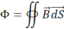
electromagnetism (Table 1-4), thermodynamics (Table 1-5) and thermal radiations
(Table 1-6) are the fundamentals for describing levitation mechanisms and
motion in general. Regarding the equations and symbols in tables 1-3, 1-4 and
1-6, the curious readers are invited to explore specialized books in the
respective areas.
Table 1‑1 Newton's laws of
motion [1], [2]
|
|
Newton's laws of motion
|
|
1st law
|
In an inertial frame of reference, an object either
remains at rest or continues to move at a constant velocity, unless acted
upon by a force.
|
|
2nd law
|
In an inertial reference frame, the vector sum of
the forces F on an object is equal to the mass m of that object multiplied by
the acceleration  of the
object: F = ma. (It is assumed here that the mass m is constant) of the
object: F = ma. (It is assumed here that the mass m is constant)
|
|
3rd law
|
When one body exerts a force on a second body, the
second body simultaneously exerts a force equal in magnitude and opposite in
direction on the first body.
|
Table 1‑2 Einstein’s postulates of special relativity
[3]
|
|
Postulates of special relativity
|
|
1st postulate
|
The laws of physics are invariant in all inertial
systems
|
|
2nd postulate
|
The speed of light in a vacuum is the same for all
observers, regardless of the motion of the light source
|
Table 1‑3 Consequences of special relativity
|
|
Consequences of special
relativity postulates
|
|
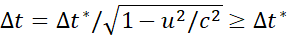
Time dilation
|
|
|
Length contraction
|
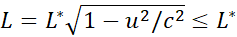
|
Table 1‑4
Laws of electromagnetism [4]
|
|
Laws of electromagnetism
|
|
Joule
|
Electric current through a conductor produces heat
|
|
Lenz
|

|
|
e is the
electromotive force (V), F the magnetic flux
|
|
Biot-Savart
|
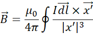
|
|
Coulomb
|
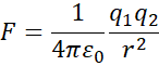
|
|
Lorentz
|
|
|
London
|
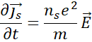
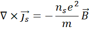
|
|
Retardation
|
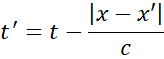
|
|
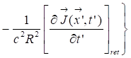
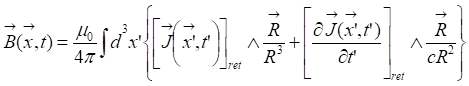
Jefimenko
|
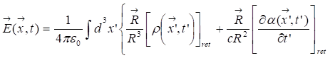 
|
See the
considered first modern book on the topic from Sadi Carnot [5] in French.
Table 1‑5
Laws of thermodynamics
|
|
Laws of thermodynamics
|
|
0th law
|
If two systems are in thermal equilibrium with a
third system, they are in thermal equilibrium with each other. This law helps
define the concept of temperature
|
|
1st law
|
When energy passes, as work, as heat, or with
matter, into or out from a system, the system's internal energy changes in
accord with the law of conservation of energy. Equivalently, perpetual motion
machines of the first kind (machines that produce work with no energy input)
are impossible
|
|
2nd law
|
In a natural thermodynamic process, the sum of the
entropies of the interacting thermodynamic systems increases. Equivalently,
perpetual motion machines of the second kind (machines that spontaneously
convert thermal energy into mechanical work) are impossible
|
|
3rd law
|
The entropy of a system approaches a constant value
as the temperature approaches absolute zero. With the exception of
non-crystalline solids (glasses) the entropy of a system at absolute zero is
typically close to zero, and is equal to the natural logarithm of the product
of the quantum ground states.
|
Table 1‑6 Thermal radiation laws
|
|
Radiation
laws
|
|
Stefan-Boltzmann
|
|
|
Wien
|

|
|
Planck
|

|
Gravity is a
long range interaction. As in electromagnetism, several attempts demonstrating
that this interaction can be shielded failed so far. Electric field cannot
escape or enter from a copper Faraday cage, while flux lines of magnetic field
do. Magnetic shields are made of high magnetic permeability materials such as
iron. In case of gravity, a hypothetical material with a high gravitational
permeability could play a role of shield.
Note at this
point, the concept of gravity shield is different from a concept of anti-gravity
device. The first is constituted with walls capable to trap gravitational waves,
but they still have a mass (the shield) submitted to gravitation, while the
anti-gravity device is rather a concept flirting with speculative physics where
its walls repulses the gravitation waves. Unfortunately, all massive bodies with
(positive) masses attract each other unless other repulsive interaction
prevails.
Let’s come back
to the concept of gravity shield. For instance why not imagine a huge
horizontal hollow pipe turning around its central axis. The mass of the pipe
submitted to gravitation must transfer information to the attractive and
massive body (Earth) of its mass while it is turning on itself. Likely the effect
of gravity inside the hollow pipe rotating at high speed could be reduced due
to the screening of gravity wave. This could be due to loss of gravitational
information exchange. This purely hypothetical exercise has been theorized in
the past, but without any convincing experimental setup so far to support it. In
the 90’s, a debate emerged with a rotating superconductor shield [6], but as discussed in 3-4, science is not only to demonstrate a
fact, a law, but consists in being reproducible at any place, at any time by
anybody having proper equipment and skills [7]. A whole area could be funded by states
in order to go in that direction. For getting funding a proof of concept must
be established at first place.
On the other
hand, proof of concepts and even working devices are capable to levitate using
the known laws of physics, as this Chapter is dedicated to.
A clear distinction is shown in Table 1‑7 between
assisted levitation from ground installation and self-levitating devices. Even
in those two families, different environmental supports are possible:
§ In fluids (Navier–Stokes
equations)
o Gas flux (see Figure 1‑1 the author performing a
ping pong levitation)
o Acoustic trapping (see Figure 1‑2 a potential
energy distribution)
o Liquid, water (see Figure 1‑3 a case of granite stone levitating above a water film)
o Ionized gas, plasma (magnetohydrodynamic, Biefeld-Brown effect)
§
Electromagnetic waves
o Electrostatics (see Figure 1‑4 a case of electrostatic
levitator in vacuum)
o Magnetostatics*
o Optics
o Radio frequency
o Superconductivity (see Figure 1‑5 for high temperature superconductors)
o Quantum electrodynamics
§
None
o Rockets
o Coupled or hybrid physics
In fluids, as well as in liquids and
in air, the magnetohydrodynamic, also noted MHD, offers the theoretical and sometimes
practical opportunities to sustain and move solid devices. As the cross-section
between fluid mechanics and electromagnetism, in particular with the Lorentz’
law, the mathematical description of MHD can be found here [8], [9]. Charge discharges and plasma
physics are mechanisms already present in Nature: active sun emitting charged
particles, solar wind and plasma streams, Earth’s magnetosphere and ionosphere.
In the technological world, plasma can be found in lighting with different
types of lamps (fluorescent, plasma displays) and in prototype controlled
fusion reactors. For both applications, the power is generally supplied from ground
installation, i.e. requiring an important amount of energy. I think it is
important to mention, here, that for levitating and moving a solid device in a
fluid with MHD, it is technically possible. Past works reported some MHD
sea-water propulsion for naval applications, as discussed by Tixador [10]. In France, Petit is a famous public
author and specialist on MHD [11], he often quoted “the silence barrier”
in opposition with the “sound barrier”. Indeed, MHD is a way to suppress the sound
barrier due to annihilation of air contact. One might wonder the amount energy necessary
for transporting a device in the sea and in air. Surely, due to Archimedes law,
less energy is required for transporting a heavy submarine in sea-water than in
air over a same distance, the submarine being heavier than air. Ionizing a
fluid and using ions to propel a device seems less constraining in a liquid
than in a gas. In air, a huge amount of energy is required at least to maintain
a steady altitude called levitation. Then an additive energy is needed for
moving in any direction. The next part 1-4 deals with the notion of impulsion
in such situation.
Theoretically, MHD propulsion is a
beautiful way to maintain a device in a steady altitude in air, or to propel in
a fluid.
Investments have been made for
military applications.
In 2018, an announcement by the
state of Russia was made concerning an ultra-fast missile, above Mach 5. Obviously,
no clear indications are available, although MHD technology might be involved.
As mentioned above, the energy embedded in a device is a key parameter for
achieving levitation. In the case of the Russian missile, a nuclear power reactor
seems to feed the propulsion. It is publicly said that the nuclear energy is
converted into heat for compressing air. It is less sure that a nuclear reactor
creates electricity with a turbine delivering a power, a voltage U and a
current I. But why not? The dream of a portative nuclear reactor is maybe real,
like a pocketreactor.
Space technologies are forwarding
a breakthrough physical concepts satisfying again a compromise between cost,
energy consumption and spacecraft speed. An interesting book treating those
topics was edited and published by the American Institute of Aeronautics and
Astronautics in 2009 [12].
In Table 1-7, cases are left
intentionally empty because of potential existent phenomena, not reported, not
known by the author. Other ways of levitations called trapping or tweezers are
not exhaustively presented here because they involve nanometer or micrometer
size objects, such as atoms, ions, aggregates, molecules, etc. Famous trapping
methods are magnetic trapping using the magnetic moment of atoms, for instance
in Bose-Einstein condensates. Other trapping techniques reported are named
Penning trap and magneto-optical trap.
Levitation is a particular case of
propulsion. Ideal levitation characterizes a floating solid object with no
physical contact as being fixed and stable in Cartesian  or spherical
 coordinates.
We get respectively during a reasonable period of time
coordinates.
We get respectively during a reasonable period of time  or
or  . Indeed in
some real levitation cases, instabilities or perturbations particularly in
fluids are met and prevent the stability conditions. Since gravity depends on
altitude, levitation is no longer an issue when the terrestrial acceleration
. Indeed in
some real levitation cases, instabilities or perturbations particularly in
fluids are met and prevent the stability conditions. Since gravity depends on
altitude, levitation is no longer an issue when the terrestrial acceleration  becomes
close to zero at high altitude. The fundamentals of propulsion physics are
known and not sophisticated where laws and principles are recognized. Tsiolkovsky
rocket equation is calculated with basic Newtonian mechanics. Solid state
physics such as superconductivity is likely the most recent one. Flotation and
levitation due to external static field forces are treated in an article [13]. There are
cheap and expensive ways to maintain levitation of a solid objects. It depends
on their weight mainly.
becomes
close to zero at high altitude. The fundamentals of propulsion physics are
known and not sophisticated where laws and principles are recognized. Tsiolkovsky
rocket equation is calculated with basic Newtonian mechanics. Solid state
physics such as superconductivity is likely the most recent one. Flotation and
levitation due to external static field forces are treated in an article [13]. There are
cheap and expensive ways to maintain levitation of a solid objects. It depends
on their weight mainly.
Table 1‑7 Ways for levitating solid objects met in Nature
and technologies
|
Support
|
Physics
domain
|
Levitation
|
|
Ground
installation
|
Embedded
system, autonomous
|
|
no
power supply
|
power
supply
|
no
power supply
|
power
supply
|
|
Fluids
|
Fluid mechanics
|
Particles in air Brownian
motion
|
Air flux
Liquid flux [14]
|
Aerostat
Submarine
|
Hummingbird
|
|
Hair dryer and ping pong
ball
|
Drone
Helicopter
|
|
Mechanics
|
|
Acoustic pressure [15]
|
|
S.A.S.E.R.
|
|
Plasma physics
|
|
|
|
M.H.D.
[8], [9]
|
|
Biefeld-Brown [16]
|
|
Electro-magnetic
waves / Photons
|
Electro-statics
|
|
Electro-static levitator [17]
|
Charged clouds
|
|
|
Magneto-statics
|
Diamagnet [18]
|
Feedback [19]
|
|
Lorentz’s force
Magnetic pressure
|
|
Paramagnet
|
|
Ferromagnet [20]
|
|
Electro-magnetism
Optics
|
|
Optical tweezers
|
|
Photon rocket
|
|
Beam-powered propulsion
|
|
Photonic laser
|
|
Electro-magnetism
Radio-frequency
|
|
Lorentz’s force:
coil above a plate
|
|
|
|
Spinning magnets: hover-board
|
|
Quantum electro-dynamics
|
Casimir effect
|
|
|
E.M. drive [21]–[24]
|
|
None
|
Mechanics
|
|
|
|
Rocket engine
|
|
Closed rocket engine
|
|
Impulsion rocket
|
|
Coupling physics
|
|
|
|
Hybrid physics
|
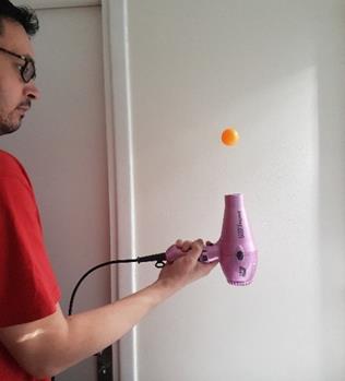
Figure 1‑1 The author performing the air flux trap
with a ping pong ball
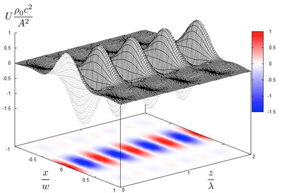
Figure 1‑2 Potential energy distribution of ultrasonic
standing wave [15]
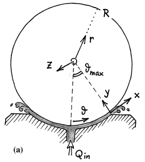
Figure 1‑3 “Kugel fontain”: a stone levitating with a
film of water [14]
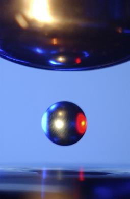
Figure 1‑4 Ti Zr-Ni alloy in an electrostatic levitator
chamber (Physics Today)
A complete list
of magnetic levitation means is shown in Table 1‑8, some comments must be
added: i/ magnetic levitation is submitted to intrinsic instability as shown
for instance in Figure 1‑6 and Figure 1‑7 with a saddle like magnetic well, ii/ in case of solid objects,
they are found sometimes in natural state, or need to be purified and
transformed with a cost of energy. The typical physical property is the
unit-less magnetic susceptibility c. Diamagnetic materials (the ideal being
the superconductors c = -1 also called the Meißner–Ochsenfeld
effect) have a negative susceptibility, while paramagnetic and ferromagnetic
materials have a positive susceptibility [25].
Susceptibilities
of typical materials are shown in Table 1‑9. Carbon atoms organized in
graphite structure show a relatively low susceptibility, C atoms are abundant.
Since a decade now that the exfoliation of highly ordered pyrolitic graphite
(HOPG) layers is a best practice for investigating electronic properties of
graphene. For the exercise, the author made the experiment of levitating a B
pencil above alternated tiny magnets, as shown in Figure 1‑8, inspired by other works [18].
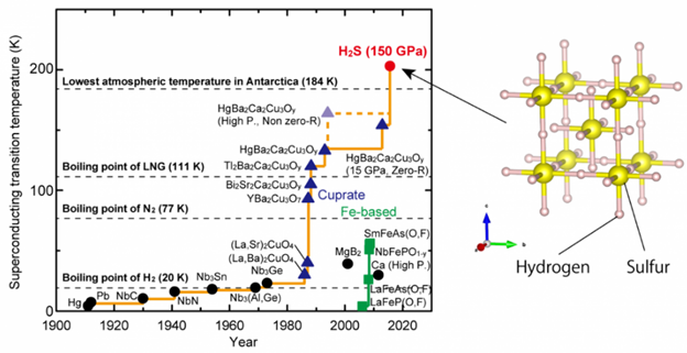
Figure 1‑5 Are room temperature superconductors possible?
[26]
Table 1‑8 Complete map of magnetic levitation and
examples
|
|
Levitating
object
|
|
Metal
|
Solid object
|
Coil / 
|
|

|
 / /
|
|

|

|
|
|
|
Ground
installation
|
Metal
|
|
|
|
[27]
|
|
coil above plate
|
|
Solid object
|
|
|
|
wip
|
wip
|
wip
|
|
|

|
|
|
[18]
|
[20]
|
wip
|
|
|
[27]
|
wip
|
wip
|
wip
|
|
Coil
|
|
|
[28]
|
|
|
[29]
|
|
Table 1‑9 Magnetic susceptibilities of different
elements [30]
|
Elements
|
(c10-9)
|
|
Elements
|
 (c10-9) (c10-9)
|
|
Ag
|
-19,5
|
|
Al
|
16,5
|
|
Bi
|
-280,1
|
|
Ti
|
153
|
|
C Graphite
|
-6
|
|
|
|
|
Cu
|
-5,46
|
|
|
|
|
In
|
-107
|
|
|
|
|
Pb
|
-23
|
|
|
|
|
Sn
|
-37
|
|
|
|
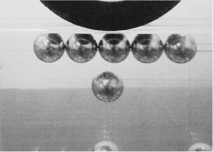
Figure 1‑6 Iron ball floating in air [20]
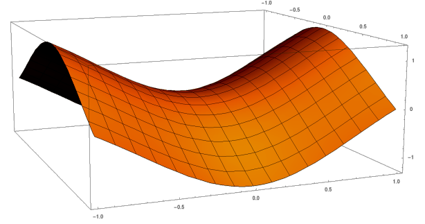
Figure 1‑7 Instable potential well (saddle like) under
static magnetic field
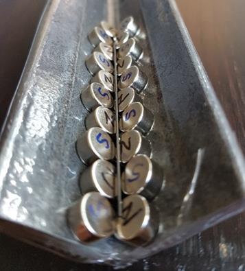
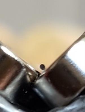
Figure 1‑8 The author performing a diamagnetic
levitation of a B pencil lead
A basic physical model of
levitation is given, it could be valid for any type of physical ways as long as
an impulsion is given. The model treats a uniform field force, a solid object
is capable of producing impulses controlled by itself. The case of
gravitational field is treated, i.e. maintaining an object in sustentation is
similar with suppressing the field force. The interest is considerable for
technological point of view, it reduces the constraints of Earth attraction
when taking off and traveling into space. Nowadays technologies of physical
thrusters offer nanonewton or micronewton forces are not able to lift an object
by itself, i.e. offering enough impulsion to its center-of-mass to counter
balance a uniform gravitational force field. The following part gives physical
parameters dedicated to the instrumentation controlling the levitation
stability. With Newton equation, time, frequency energy and power
considerations are given. The model opens routes toward design of levitating
devices.
A body with mass m in the vicinity
of massive body such our Earth is submitted to attraction force described with
Newton equation:
where is the
acceleration depending on the massive body mass, gravitational constant and
distance between two bodies, on Earth  . The free
fall is perfectly described using the Equation 1.1. Now consider the body capable
of giving an impulse force in the direction opposite to attraction.
. The free
fall is perfectly described using the Equation 1.1. Now consider the body capable
of giving an impulse force in the direction opposite to attraction.
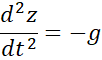
Along an axis z with 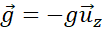 , as shown in
Figure 1‑9, in free fall
the acceleration is noted
, as shown in
Figure 1‑9, in free fall
the acceleration is noted
|
|
Equation 1.2
|
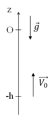
Figure 1‑9 Free fall axis
Initial conditions are
§
rest position at height 
§
impulse against gravity direction at speed 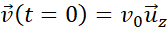
Both speed and acceleration can be
calculated
|
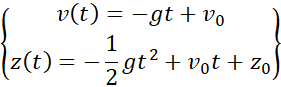
|
Equation 1.3
|
Time when  is then
|
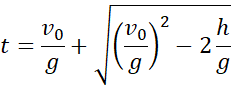
|
Equation 1.4
|
Moreover the principle of energy
conservation gives us that
|
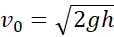
|
Equation 1.5
|
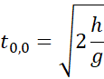
Therefore the time when both speed
and height are at equal zero
The time in Equation 1.6 is nothing else the time when
the solid object reaches a new rest position before falling in free fall, as
shown in Figure 1‑10. The
principle of apparent levitation is to give an impulse at each new rest
position and in such way that  is very
small. It is a pseudo levitation that still looks like a levitation on small
time scales, while on long time scale the object moves up.
is very
small. It is a pseudo levitation that still looks like a levitation on small
time scales, while on long time scale the object moves up.
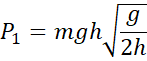
From quantitative point of view,
the calculation of power necessary for insuring one jump is:
where  is the
energy coming the pulse of force in one period, ie it is the energy necessary
to elevate the object from
is the
energy coming the pulse of force in one period, ie it is the energy necessary
to elevate the object from  to
to  , and
, and  the
frequency of energy pulse.
the
frequency of energy pulse.
Note the is equal to
kinetic or potential energy  in amplitude
range of height h. Therefore Equation 1.7 becomes:
in amplitude
range of height h. Therefore Equation 1.7 becomes:
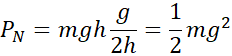
Now the power related in 1 second
when N pulses are submitted such as  , therefore
the power per second unit is
, therefore
the power per second unit is 
Figure 1‑10 Apparent and pseudo-stable levitation
It is noticeable to see that the power does not depend
on . In this model, the pseudo-levitation is due to the
choice of giving an impulse at each new rest position, in the end the object
rises. A better levitation case would consist in leaving the object falling
down to the position  , i.e. the initial position, as shown in Figure 1‑11.
There, a new energy pulse against gravity is not enough to rise the object
again because of the gained kinetic energy
, i.e. the initial position, as shown in Figure 1‑11.
There, a new energy pulse against gravity is not enough to rise the object
again because of the gained kinetic energy  coming from the free fall. Double of energy
  is required for i) suppressing the kinetic energy
coming from the free fall, ii) giving impulse to go from to .
is required for i) suppressing the kinetic energy
coming from the free fall, ii) giving impulse to go from to .
In the end the power calculation for one period of
impulse is equal to Equation 1.8 because both time and energy doubled. Finally, the
power over N impulses created during one second is equal to Equation 1.9.
Since gravity and its acceleration depend on the
geophysics, a local acceleration must be measured in real-time in order to
adjust a stable levitation.
Ideal thrusters
not losing weight are still speculative, however, in the next chapter we will
go through original ideas which have been reported in public cultures, in
patents, comics, pseudo-scientific blogs, etc.
Figure 1‑11 Stable levitation model
‘There is no exquisite beauty (...)
without some strangeness in the proportion’
Edgar Poe to Lord Verulam
Sapere
Aude
‘Dare
to know’
Horace
(Epistles, I, II, 40)
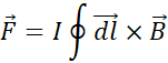
2-1 Lorentz’ force
The famous
Lorentz equation giving the force F exerted by a magnetic field B
on a current I circulating in a conducting wire.
The situation
capable to naively create a thrust is to place a magnet having a magnetic field
B perpendicular to a metallic wire having a current I, as shown
in Figure 2‑1. The
question now is to ask ourselves if the rigid device magnet-wire can move in
one direction.
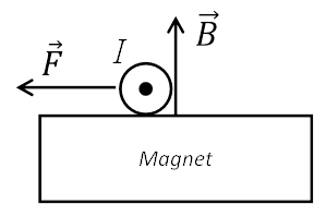
Figure 2‑1 Permanent magnet creates a force F in
a conductor with a current I
In the device
magnet-wire the asymmetry stands only in the geometry, the magnetic field B
emitted by the magnet creates a force on the wire and inversely the current I
circulating in the wire.
Having
experimented by myself I can confirm no displacements were visible. Here again
if the heat losses were asymmetrical between magnet and wire, likely a full
thermodynamic treatment could demonstrate that the device creates a thrust.
Another idea is
the magnetic pressure exerted on a conical coil. The magnetic pressure is an
important concept when designing and building solenoids with elevated magnetic
field. A long cylindrical solenoid, as shown in Figure 2‑2, having N’ spires
per meter is flowed by a current I. Then the current per length unit is N’I.
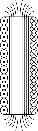
Figure 2‑2 Cylindrical coil represented with magnetic
flux lines
The metallic wound
wire constituting the cylindrical coil has diameter a. In the coil, the
magnetic field is axial and uniform
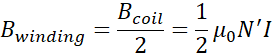
Having a null
magnetic field outside the coil, inside the winding, the average magnetic field
B is half of term given in Equation 2.2.
|
|
Equation 2.3
|
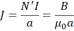
However, inside
the winding, the magnetic field B is axial and the current density is
tangential. Then, the volume force density taken from Lorentz Equation 2.1 is equal at  (you can check
that the dimensions are indeed N/m3 i.e. a force in Newton per volume unit) and is oriented radially outside
the coil. The volume force density of magnetic field exerted on the winding is
like having a gas pressure, like if a gas under pressure was trapped inside the
coil. What is the value of this pressure? The volume force density F’ is
given by JB where
(you can check
that the dimensions are indeed N/m3 i.e. a force in Newton per volume unit) and is oriented radially outside
the coil. The volume force density of magnetic field exerted on the winding is
like having a gas pressure, like if a gas under pressure was trapped inside the
coil. What is the value of this pressure? The volume force density F’ is
given by JB where
|
|
Equation 2.4
|
Then the volume force
density (N/m3) at the winding is equal at
|
|
Equation 2.5
|
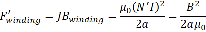
In the end the
magnetic pressure (N/m2) exerted on the wire having a diameter a is
equal at
|
|
Equation 2.6
|
Note that the
pressure depends on the squared of magnetic field. Note also that we have
considered a null magnetic field outside the solenoid. Is the magnetic pressure
significant? Let’s take B = 1 T. Then the pressure is equal at
|
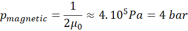
|
Equation 2.7
|
Usually
designing high magnetic field coils require a care for preventing mechanical
deformation with wires as well as made of copper or superconductive materials.
In the case of a
conical coil, as shown in Figure 2‑3, we can launch the question, what is the effect of magnetic
pressure on the coil. Does the pressure exerted on the winding trigger a thrust
toward the direction of the little base of the cone? This would be possible if
the magnetic force is indeed normal (perpendicular) to the coil surface. For
now I do not have a mathematical demonstration to show that the coil does move
or not toward the little base of the cone. What is certain is that the magnetic
field amplitude decreases when going from the little base to the large base of
the cone.
However, if we
can come back to the analogy of gas pressure contained in a conical balloon.
Does a conical balloon move toward its small base cone? Surely not.
Note that the
conical shape is met in device called ‘RF resonant cavity thruster’ designed by
Roger Shawyer. Interesting and less interesting communications are now in the
public domain [21-22], [24], [31-36]. Again, nano, micro
newton are involved here. Think big, start small.
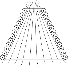
Figure 2‑3 Conical coil represented with magnetic flux
lines
In this part, I would like to entertain the reader
interested in propulsion techniques which do not expel chemicals or ions. Some
people call this technology ‘closed systems’ if they indeed only use internal
and closed mechanical motion and if they do not interact with the environment
by expelling mass or heat (radiation, conduction or convection). Closed system
must mean also adiabatic system, this is the discussion of the last chapter.
Closed systems seem to violate the principle of momentum conservation. It seems
naive at first place to treat about this subject, however, tenths of honest
people developed the wackiest devices sometimes patented. The run for money
nowadays makes lose all notions of physics.
Those closed systems are in opposition with open
systems having an interaction with the environmental space. I will demonstrate
that ideal closed mechanical systems are impossible to use as a propulsion and
thruster technology. However, real systems encounter mechanical frictions
leading to heat loss and this opens a possible way to explore for applications.
The conservation of energy might supplant conservation of momentum as discussed
in the last chapter.
To put the context, let’s start to draw a simple
picture. A fisherman on a little boat lost his paddles. Fortunately, his bucket
water filled is plenty of big alive fish. Then, he has the idea to throw them
away from the boat in one opposite direction of his wished target on waterside.
By the way, he noticed the boat took some momentum when he thrown very hard.
The first example of propulsion without propellant
appearing in patents having sometimes several tenths of pages starts from the
following idea: the current chemical rockets use a propulsion of ejected matter
into space, so why not recuperating the matter into a closed circuit, for
eventually decelerate it and reaccelerate. Gyroscope thruster also starts with
similar considerations.
In order to demonstrate that it does not work, I took
the example of two masses M that I launch in the back of a ship creating so a
thrust in front of the ship. The two masses would be recuperated on two
opposite circular circuits or rails guiding the motion in such way that the
ship still keeps a rectilinear direction.
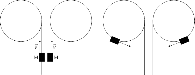
Figure 2‑4 Schematic of two masses launched in 2 symmetrical rails
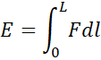
The thrust is the force that accelerated masses
exchange with the ship, the kinetic energy is equal to the integral of the
force F on the length L on which force is exerted:
|
|
Equation 2.8
|
According to Figure 2‑4 and
Figure 2‑5, the mass M
starts its curved path at a point x = r and y = 0 at a speed V,
then the mass reaches α after a time  .
.
|
|
Equation
2.9
|
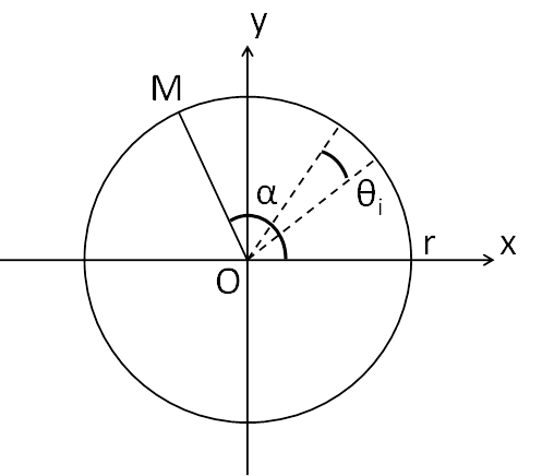
Figure 2‑5 Circle on which mass the M stays confined in
closed circuit
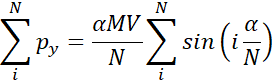
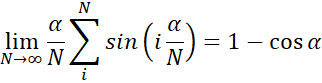
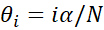
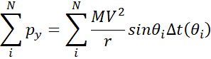
where N is the
number of position that will be integrated along the axis y, I will calculate
the contribution of initial force on the y component, for that I use the
quantity of motion  .
.
|
|
Equation 2.10
|
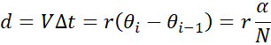
Concretely, it
means that the mass M transfers both energy and momentum along axis Oy.  is the time
that the mass M travels on the circle the angle
is the time
that the mass M travels on the circle the angle  . Let’s
define d a being the distance between
. Let’s
define d a being the distance between  and
and  on the
circle, then the following can be written:
on the
circle, then the following can be written:
|
|
Equation 2.11
|
Then the
quantity of motion is written:
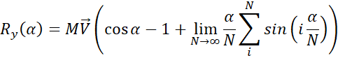
The resultant of
momentum quantity  along the y
axis is expressed as the sum of initial momentum quantity
along the y
axis is expressed as the sum of initial momentum quantity  plus the
reaction of mass M on the curvature which is Equation 2.12 with N going to infinity, plus
the contribution of mass M when stopping abruptly at the position
plus the
reaction of mass M on the curvature which is Equation 2.12 with N going to infinity, plus
the contribution of mass M when stopping abruptly at the position  .
.
|
|
Equation 2.13
|
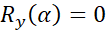
A mathematical numerical software can show
that
Therefore the resultant becomes null:
|
|
Equation 2.15
|
It can be
comforting, intuitive and logical for some, or, crazy, insane and impossible
for others, but the fact is it is not possible to use gyroscopes, closed
circuit, for moving a full body without losing its mass.
However.
And now it is
becoming interesting.
If some losses are
generated when our system of two masses follows the circular path, then the Equation 2.14 is no longer valid. The
momentum would be not transferred entirely into the device, but would be partly
lost in the loss mechanism. The losses can have different origins, they can be
mechanical friction in case of mechanical contact or eddy current heating in
case of magnetic rails, etc. In any cases, the losses are a conversion of mechanical
momentum into heat. In case of adiabatic closed system, the internal
temperature increases, dissipation is then recommended by conduction (and
convection) and radiation. Therefore, the thermodynamics physics enters here as
a trigger for alternative ways for thrust. As a consequence, such system is
partially closed. It is mechanically closed but because heat exchange such as
infrared radiations must exit for preventing the adiabatic system to increase
in temperature.
‘Words exist because of meaning.
Once you've gotten the meaning, you can forget the
words.
Where can I find a man who has forgotten words so I
can talk with him?’
Zhuangzi (369-286 BC)
Labor omnia improbus vincit
‘A hard work defeats everything’
Virgil (Georgics, I, 144-145)
3-1 One case: Coil-Disc device
In Chapter 2 we have seen that the
action-reaction principle works perfectly for mechanical systems and that any
tricks to circumvent this specific law of Nature is not possible. In the same chapter,
we have seen a non-contact interaction based on magnetic interaction, and the
same conclusion remains, for every distant or retarded interaction a counter
interaction exists. However, a bias exists that is to create an asymmetry in
the losses that are frictions in mechanics, joule heating in metals submitted
by electromagnetic waves and eddy currents. As much as surprising it might be,
this the latter one we want to enhance in order to create a breaking in the
action-reaction principle.
In this Chapter the case of an
electromagnetic actuator creating a non-contact force on a disc is taken. This
choice is not fully arbitrary since it has been theorized, tested and published
in peer review journals. The device Coil-Disc is taken as an illustration of
the demonstration, but any other device satisfying the breaking by creating
asymmetrical losses is satisfying too.
In the following three lines, we
can see the basic notions:
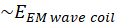
1. Electromagnetic actuator and the Lenz’s law: electromagnetic energy
2.
Lorentz force: mechanical work
3. Thermal dissipation: Joule and thermal losses
Conservation of mechanical
momentum is possible when the term 3. is null and is not possible when losses
are present. Therefore conservation of energy supplants the action-reaction law.
As shown in Figure 3‑1, in thermodynamics:
§
the open system stands for open exchange of
matter and energy with the environment
§
the closed system stands for open exchange of
energy but not for the matter
§
the isolated system stands no exchange of energy
and matter to the environment
In vacuum the only way to expel
heat is an emissive radiation likely in the infrared spectrum from the black
body radiation. This is not in any case comparable to a laser thruster which is
directional. Here the radiation of the device is required for preventing an
internal heating, and is preferably chosen to be isotropically evacuated for
avoiding temperature rise on the surface.
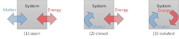
Figure 3‑1 Definitions of (1) open, (2) closed, and
(3) isolated systems
The two basic postulates to keep
in mind are energy conservation and momentum conservation.
The famous experiment of the jumping ring can be
practiced even at home when plugging a solenoid to the electrical network,
illustrated in Figure 3‑2. There
are plenty of videos on the internet showing that a ring placed in front of a
solenoid coil filled with an iron core, the ring jumps away from the coil. Be
aware for risks of electrical accident when performing the experiment at home. The
fast transient current flowing in the coil is responsible for a fast transient
magnetic flux in the ring, itself opposed in direction to the induced one. Now
the idea is to attach rigidly both coil and ring together. As discussed in
Chapter 3, the only way to reduce the counter force coming from the ring is to
increase its losses from joule heating.
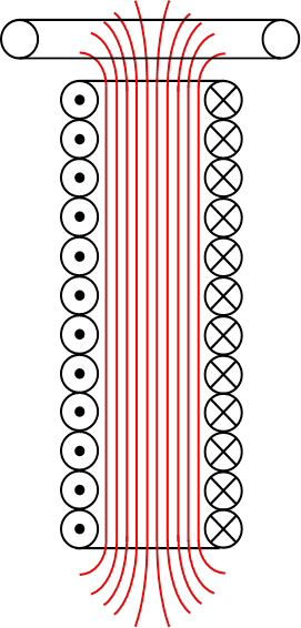
Figure 3‑2 Coil-ring device with magnetic field lines
In one hand, when cooling down the
ring its resistance becomes much smaller, then the induced electromotive and
Lorentz forces becomes much higher and the jump becomes much higher. The trick
to use a copper ring at room temperature is to guarantee heat dissipation
therefore energy loss. For a given shape of impulse electromagnetic wave coming
from the coil, the losses in the copper ring must be enhanced in order to
reduce the amplitude of waves coming back from the ring. In the meantime the
jump becomes smaller. A full model has been built, simulated and published [37]. Further a test device has been tried
and showed success [29]. Lively comments came immediately after
the publication of the results. The major criticism is the fact the Earth
magnetic field was not properly shielded during the experiment. In fact, in the
equation of motion, the device is sensitive on fast changing magnetic field and
not to a constant magnetic fields such as the Earth one. Note that the model
itself has not been so far contradicted, on the contrary. Another aim of this
Chapter is to eventually challenge the model.
In the following we will discuss
the device coil-disc instead of coil-ring. In the model we assume a disc as
being an assembly of tiny rings stuck the ones against the others, as shown in Figure 3‑3.
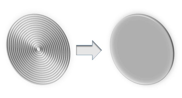
Figure 3‑3 Assumption of a disc as being discretized with
multi-rings
Let’s write now the equation of
energy conservation. First the energy emitted by the coil can be described as
the sum of the two sides.
The first term of Equation 3.1 is the energy lost in vacuum the
empty side of the coil. The second term of Equation 3.1 is the energy coming the coil
reaching the disc  while a tiny
part
while a tiny
part  can be lost
in vacuum too if the device is not magnetic tight.
can be lost
in vacuum too if the device is not magnetic tight.
Now let’s give a description of
the first term which is the parameter for driving energy balance between
mechanic work  , heat
dissipation
, heat
dissipation  , and
counter-force coming reemitted electromagnetic waves from the disc to the coil
, and
counter-force coming reemitted electromagnetic waves from the disc to the coil  . Indeed the
first term of Equation 3.2 is
the sum of different energies:
. Indeed the
first term of Equation 3.2 is
the sum of different energies:
Indeed the electromagnetic waves
coming from the coil create eddy currents on the metallic disc, and those
currents submitted to magnetic field, the Lorentz force creates a work, the
first term of Equation 3.3. In
the same time, eddy currents create joule heating (black body radiation), the
second term of Equation 3.3. Eddy
currents might reemit electromagnetic waves with an amplitude depending on the
eddy currents, third term of Equation 3.3, which is responsible of the counter force, and a counter work to
the coil  .
.
|

|
Equation 3.4
|
Similar reasoning as stated above
can be done.
|

|
Equation 3.5
|
As for the transmission from coil
to disc, now let’s describe the energy process from disc to coil.
Now having put the basic
fundamentals of energy exchanges, the only way to produce a useful work in the
coil-disc device is to have the following condition satisfied.
We can go even further by
establishing another condition  .
.
When looking at equations, from Equation 3.3 to Equation 3.6, we clearly see that is smaller
and is a fraction of  . However
this does not mean that . The weight
of the three terms in the master Equation 3.3 is not known. An exercise is to assess the contribution of each
term of heat dissipations and
. However
this does not mean that . The weight
of the three terms in the master Equation 3.3 is not known. An exercise is to assess the contribution of each
term of heat dissipations and  . When having
resistive materials such copper, aluminum at room temperature, we can assume
some heat dissipations. In opposite when having low resistive materials at low
temperatures (resistive or superconducting materials), the heat dissipations
become negligible.
. When having
resistive materials such copper, aluminum at room temperature, we can assume
some heat dissipations. In opposite when having low resistive materials at low
temperatures (resistive or superconducting materials), the heat dissipations
become negligible.
In Table 3-1 different situations of resistive
materials are summarized. Starting from normal metals such as copper, aluminum
for resistive metals at room temperatures, to low resistive metals generally
realized at low temperatures either with normal metals or superconductors. Remind
again that the term is the energy dissipated in the coil coming from the
counter electromagnetic wave. The easiest case to realize in a laboratory is
the case #1 where no constraining cryogenic technologies are required. The
cases #2, #3 and #4 require cryogenic technologies and all the drawbacks and
difficulties appear. On the other hand, the chance to observe any total work or
displacement is small in the case #1 if not having very sensitive equipment
measuring tiny displacements. In summary the most favorable situation is
qualitatively the case #2 where the is expected to be larger than . The case #2 is a favorable situation for creating a thermal
asymmetry in the system.
Whatever the cases of the Table 3-1 to experiment, to
improve, to challenge, what matters in the end for a final user is to get the Equation 3.7
satisfied not only on short time scales like the time for the electromagnetic
wave to travel forward and back but on long time scales, as long as the coil
emits transient electromagnetic waves. A cross-talk between newly reemitted
wave and previous back waves must be considered.
Table 3‑1 Qualitative assessment of different cases
where heat dissipation and work are confronted in the device coil-disc
|
Case
|
Disc
|
Balance
sheet
Equation 3.3
|
Coil
|
Balance
sheet
Equation 3.6
|
|
#1
|
Resistive
|

|
Resistive
|

|
|
#2
|
Low
resistive
|


|
Resistive
|
|
|
#3
|
Resistive
|
|
Low
resistive
|


|
|
#4
|
Low
resistive
|
|
Low
resistive
|
|
A gedankenexperiment, proposal of
experiments, preliminary results and first exchanges via normal communications,
erratum and corrections are already available to the public domain [29], [38–41]. The only valid and solid
hypothesis is the energy conservation in the coil-disc system between provided
electrical energy, work and heat dissipation. The latter coming from joule
losses triggers the asymmetrical forces [37], [42]. Route of improvement is to
increase the work which in turns balances joule losses. This technology turns out
to be a way to produce a brutal acceleration by a short pulse of force also
called impulse, necessary to get levitation as stated in Chapter 1.
However, for lifting heavy loads, both
an important electrical generator and an optimized design for dissipating heat
are required.
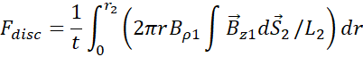
The force
expression on the disc after a first wave travel coming from the coil was given
in the references [29], [37], [40], and was confronted with
experimental data.
where t, r2, r, Br1, Bz1, S2 and L2 are respectively, the disc thickness, the disc and integration
radius, the radial and axial magnetic field components at the extremity of the
coil, the disc area and the ring integration inductance. Experiments were
performed with an angle between the geological north-south line and the coil
axis at 15°. The disc was oriented to the south-east and the coil to the
north-west. Measurements were performed at Latitude: 46.6592 and Longitude: 0.3596.
A magnetic field component (along Bz1) such as the Earth magnetic
field which is not time dependent within the time scale of experiments does not
create a force on the disc since only the time dependent fields contribute into
the force of Equation 3.8. This
explanation can close the ‘Earth magnetic field controversy’ related to the
measurements. The issue of surrounding environment of the coil-disc system
contributing to the total thrust might be raised when taking into account
sources of artifacts, such as mirror charging
effects. A care was taken in order to prevent proximity mirror effects by using
an immediate environment made of wood.
Since involved
forces are very tiny, several techniques are reported to be efficient [36], [43–66] as soon as are satisfied the
following conditions: a proper calibration, a noise-free environment. Finally,
the confidence of the experimenter for not recording stray signals might be
important as well.
As discussed in
the previous parts, heat must be released from the system. In vacuum, radiation
dominates therefore in this part we remind the physics of radiation.
Heat comes from
the induced current and is given by 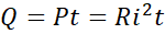 .
.
Beside the final
temperature  can be
calculated with
can be
calculated with 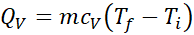 where
where  ,
,  and
and  are
respectively the mass, mass heat capacity and initial temperature in Kelvin.
are
respectively the mass, mass heat capacity and initial temperature in Kelvin.
Wien law gives a
relationship between the wavelength  with the
highest emission from a perfect black body and the temperature, their product
is constant.
with the
highest emission from a perfect black body and the temperature, their product
is constant.
|
|
Equation 3.9
|
For instance, at
300 K,  , the
emission is in the infrared spectrum.
, the
emission is in the infrared spectrum.
Stefan-Boltzmann
law gives the thermal flux (thermal power) emitted by a surface S of a black
body at a temperature T
|

|
Equation 3.10
|
where is the Stefan-Boltzmann constant. The surface flux emitted by a black body
at a temperature is then 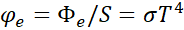 .
.
In this last
part, the underlying treated notions are about scientific integrity and repeatability
in science. The sad story of innovative concepts in physics particularly
advanced ones is that some:
Ø
cannot be submitted to experimental validations
because of lack of appropriate technical instruments at one moment of history
Ø
cannot be repeated by other peers showing negative
results or positive results
Ø
can be repeated by other peers showing negative results
or positive results.
A knowledge in
theoretical and experimental sciences is shared and promoted via edition of an academic
book, publication of an article with an independent and specialized referee,
and this whatever the area of science. Tacit terms of reproducibility in
experimental physics are [67]:
1.
Initial skepticism on the
facts (thanks to Pyrron)
2.
Realism on principle
3.
Methodological materialism
4.
Rationality (and logics).
The physical
world Re is the sum of different sets. They are perceptible world P (even
distorted), plus a fraction n (n<1) of imaginary I world, plus an
imperceptible C world, plus a not imaginable G world. Those sets might have
dependence, for instance, imperceptible C world can superpose a part of a not
imaginable G world. Also P is accessible with human senses, instruments
converting non accessible signals by humans into accessible.
[1] I. Newton, “The mathematical
principles of natural philosophy (Vol. I),” Oxford Univ., p. 352, 1728.
[2] I.
Newton, “The mathematical principles of natural philosophy (Vol. II),” Oxford
Univ., 1728.
[3] A.
Einstein, “Zur Elektrodynamik bewegter Körper,” Ann. Phys., pp. 891–921,
1905.
[4] J.
D. Jackson, Classical Electrodynamics, John Wiley. New York, 1999.
[5] S.
Carnot, Réflexions sur la puissance motrice du feu et sur les machines propres
à développer cette puissance. 1824.
[6] E.
Podkletnov and R. Nieminen, “A possibility of gravitational force shielding by
bulk YBa2Cu3O7−x superconductor,” Phys. C Supercond., vol. 203,
no. 3–4, pp. 441–444, Dec. 1992.
[7] G.
Hathaway, B. Cleveland, and Y. Bao, “Gravity modification experiment using a
rotating superconducting disk and radio frequency fields,” Phys. C
Supercond., vol. 385, no. 4, pp. 488–500, Apr. 2003.
[8] R.
J. Hosking and R. L. Dewar, Fundamental Fluid Mechanics and
Magnetohydrodynamics. Singapore: Springer Singapore, 2016.
[9] A.
Piel, Plasma Physics. Berlin, Heidelberg: Springer Berlin Heidelberg,
2010.
[10] P.
Tixador, “Magnetic levitation and MHD propulsion,” J. Phys. III, vol. 4,
no. 4, pp. 581–593, Apr. 1994.
[11] J.-P.
Petit, J. Geffray, and F. David, “MHD hypersonic flow control for aerospace
applications,” in 16th AIAA/DLR/DGLR International Space Planes and
Hypersonic Systems and Technologies Conference, 2009, pp. 1–19.
[12] M.
G. Millis and E. W. Davis, Frontiers of Propulsion Science. Reston ,VA:
American Institute of Aeronautics and Astronautics, 2009.
[13] E.
H. Brandt, “Levitation in Physics,” Science (80-. )., vol. 243, no.
4889, pp. 349–355, Jan. 1989.
[14] J.
H. Snoeijer and K. van der Weele, “Physics of the granite sphere fountain,” Am.
J. Phys., vol. 82, no. 11, pp. 1029–1039, Nov. 2014.
[15] Y.
Ochiai, T. Hoshi, and J. Rekimoto, “Three-Dimensional Mid-Air Acoustic
Manipulation by Ultrasonic Phased Arrays,” PLoS One, vol. 9, no. 5, p.
e97590, May 2014.
[16] M.
Einat and R. Kalderon, “High efficiency Lifter based on the Biefeld-Brown
effect,” AIP Adv., vol. 4, no. 7, p. 077120, Jul. 2014.
[17] W.
Rhim et al., “An electrostatic levitator for high‐temperature containerless
materials processing in 1‐g,” Rev. Sci. Instrum., vol. 64, no. 10,
pp. 2961–2970, Oct. 1993.
[18] V.
Koudelkova, “How to simply demonstrate diamagnetic levitation with pencil
lead,” Phys. Educ., vol. 51, no. 1, p. 014001, Jan. 2016.
[19] A.
J. Sangster, Fundamentals of electromagnetic levitation : engineering
sustainability through efficiency, vol. 24. 2012.
[20] S.
Sasaki, I. Yagi, and M. Murakami, “Levitation of an iron ball in midair without
active control,” J. Appl. Phys., vol. 95, no. 4, pp. 2090–2093, Feb.
2004.
[21] M.
Tajmar and G. Fiedler, “Direct Thrust Measurements of an EMDrive and Evaluation
of Possible Side-Effects,” in 51st AIAA/SAE/ASEE Joint Propulsion Conference,
2015, no. September, pp. 1–10.
[22] P.
Grahn, A. Annila, and E. Kolehmainen, “On the exhaust of electromagnetic
drive,” AIP Adv., vol. 6, no. 6, p. 065205, Jun. 2016.
[23] M.
Monette, “The SpaceDrive Project-Thrust Balance Development and New
Measurements of the Mach-Effect and EMDrive Thrusters,” no. October, 2018.
[24] D.
Brady, H. White, P. March, J. Lawrence, and F. Davies, “Anomalous Thrust
Production from an RF Test Device Measured on a Low-Thrust Torsion Pendulum,”
in 50th AIAA/ASME/SAE/ASEE Joint Propulsion Conference, 2014, pp. 1–21.
[25] M.
Gezlaff, Fundamentals of Magnetism. Berlin, Heidelberg: Springer Berlin
Heidelberg, 2008.
[26] M.
Einaga et al., “Crystal structure of the superconducting phase of sulfur
hydride,” Nat. Phys., vol. 12, no. 9, pp. 835–838, Sep. 2016.
[27] D.
G. Henderson et al., “Hoverboard which generates magnetic lift to carry
a person,” 2015.
[28] E.
Beaugnon and R. Tournier, “Levitation of organic materials,” Nature,
vol. 349, no. 6309, pp. 470–470, Feb. 1991.
[29] D.
S. H. Charrier, “Micronewton electromagnetic thruster,” Appl. Phys. Lett.,
vol. 101, no. 3, p. 034104, Jul. 2012.
[30] H.
Stöcker, F. Jundt, and G. Guillaume, Toute la Physique, Dunod. 1999.
[31] T.
Lafleur, “Can the quantum vacuum be used as a reaction medium to generate
thrust?,” Arxiv, pp. 1–22, Nov. 2014.
[32] R.
Shawyer, “Second generation EmDrive propulsion applied to SSTO launcher and
interstellar probe,” Acta Astronaut., 2015.
[33] M.
E. McCulloch, “Testing quantised inertia on the emdrive,” EPL (Europhysics
Lett., vol. 111, no. 6, p. 60005, Sep. 2015.
[34] J.
J. Rodal, “NASA’ s microwave propellant-less thruster anomalous results :
consideration of a thermo-mechanical effect,” Rodal, José J, no. August,
2015.
[35] H.
White et al., “Measurement of Impulsive Thrust from a Closed
Radio-Frequency Cavity in Vacuum,” J. Propuls. Power, pp. 1–12, Nov.
2016.
[36] C.
P. Duif, “An improved method to measure microwave induced impulsive forces with
a torsion balance or weighing scale,” Tech. Rep., no. June, 2017.
[37] D.
S. H. Charrier, “Loss of linear momentum in an electrodynamics system: from an
analytical approach to simulations,” Prog. Electromagn. Res. M, vol. 13,
pp. 69–82, 2010.
[38] D.
P. Goodwin, “A possible propellantless propulsion system,” in AIP Conference
Proceedings, 2001, vol. 552, pp. 976–978.
[39] T.
Lafleur, “Comment on ‘Micronewton electromagnetic thruster’ [Appl. Phys. Lett.
101 , 034104 (2012)],” Appl. Phys. Lett., vol. 105, no. 14, p. 146101,
Oct. 2014.
[40] D.
S. H. Charrier, “Erratum: ‘Micronewton electromagnetic thruster’ [Appl. Phys.
Lett. 101 , 034104 (2012)],” Appl. Phys. Lett., vol. 105, no. 14, p.
149902, Oct. 2014.
[41] D.
S. H. Charrier, “Response to ‘Comment on “Micronewton electromagnetic
thruster”’ [Appl. Phys. Lett. 105 , 146101 (2014)],” Appl. Phys. Lett.,
vol. 105, no. 14, p. 146102, Oct. 2014.
[42] D.
S. H. Charrier, “Frequency spectrum analysis on the force contribution in a
micronewton electromagnetic thruster,” in APS March Meeting 2016, 2016,
p. 1.
[43] J.
K. Ziemer, “Performance Measurements Using a Sub-Micronewton Resolution Thrust
Stand,” 27th Int. Electr. Propuls. Conf., 2001.
[44] A.
R. Wong, A. Toftul, K. A. Polzin, and J. B. Pearson, “Non-contact thrust stand
calibration method for repetitively pulsed electric thrusters,” Rev. Sci.
Instrum., vol. 83, no. 2, p. 025103, Feb. 2012.
[45] D.
Zhang, J. Wu, R. Zhang, H. Zhang, and Z. He, “High precision micro-impulse
measurements for micro-thrusters based on torsional pendulum and sympathetic
resonance techniques,” Rev. Sci. Instrum., vol. 84, no. 12, p. 125113,
Dec. 2013.
[46] J.
Soni, J. Zito, and S. Roy, “Design of a microNewton Thrust Stand for Low
Pressure Characterization of DBD Actuators,” in 51st AIAA Aerospace Sciences
Meeting including the New Horizons Forum and Aerospace Exposition, 2013,
no. July, pp. 1–13.
[47] Z.
He, J. Wu, D. Zhang, G. Lu, Z. Liu, and R. Zhang, “Precision electromagnetic
calibration technique for micro-Newton thrust stands,” Rev. Sci. Instrum.,
vol. 84, no. 5, p. 055107, May 2013.
[48] J.
E. Polk et al., “Recommended practices in thrust measurements,” in The
33rd International Electric Propulsion Conference, 2013, pp. 1–24.
[49] J.
Soni and S. Roy, “Design and characterization of a nano-Newton resolution
thrust stand,” Rev. Sci. Instrum., vol. 84, no. 9, p. 095103, Sep. 2013.
[50] M.
Kühnel, M. Rivero, C. Diethold, F. Hilbrunner, and T. Fröhlich, “Precise
tiltmeter and inclinometer based on commercial force compensation weigh cells,”
Conf. IMEKO Int., no. FEBRUARY, pp. 1–5, 2014.
[51] J.
Lun and C. Law, “Direct thrust measurement stand with improved operation and
force calibration technique for performance testing of pulsed micro-thrusters,”
Meas. Sci. Technol., vol. 25, no. 9, p. 095009, Sep. 2014.
[52] G.
Hathaway, “Sub-micro-Newton resolution thrust balance,” Rev. Sci. Instrum.,
vol. 86, no. 10, p. 105116, Oct. 2015.
[53] S.
Chakraborty, “An Electrostatic Ion-guide and a High-resolution Thrust-stand for
Characterization of Micro-propulsion Devices,” THESIS, vol. 6645, 2015.
[54] S.
M. Merkowitz, P. G. Maghami, A. Sharma, W. D. Willis, and C. M. Zakrzwski, “A μNewton
thrust-stand for LISA,” Class. Quantum Gravity, vol. 19, no. 7, pp.
1745–1750, Apr. 2002.
[55] L.
Liu, X. Ye, S. C. Wu, Y. Z. Bai, and Z. B. Zhou, “A low-frequency vibration
insensitive pendulum bench based on translation-tilt compensation in measuring
the performances of inertial sensors,” Class. Quantum Gravity, vol. 32,
no. 19, p. 195016, Oct. 2015.
[56] S.
Chakraborty, D. G. Courtney, and H. Shea, “A 10 nN resolution thrust-stand for
micro-propulsion devices,” Rev. Sci. Instrum., vol. 86, no. 11, p.
115109, Nov. 2015.
[57] F.
G. Hey, A. Keller, C. Braxmaier, M. Tajmar, U. Johann, and D. Weise, “Development
of a Highly Precise Micronewton Thrust Balance,” IEEE Trans. Plasma Sci.,
vol. 43, no. 1, pp. 234–239, Jan. 2015.
[58] S.
Vasilyan, M. Rivero, J. Schleichert, B. Halbedel, and T. Fröhlich,
“High-precision horizontally directed force measurements for high dead loads
based on a differential electromagnetic force compensation system,” Meas.
Sci. Technol., vol. 27, no. 4, p. 045107, Apr. 2016.
[59] J.
E. Polk et al., “Recommended Practice for Thrust Measurement in Electric
Propulsion Testing,” J. Propuls. Power, vol. 33, no. 3, pp. 539–555, May
2017.
[60] M.
Gamero-Castaño, “A torsional balance for the characterization of microNewton
thrusters,” Rev. Sci. Instrum., vol. 74, no. 10, pp. 4509–4514, Oct.
2003.
[61] K.
a. Polzin, T. E. Markusic, B. J. Stanojev, A. DeHoyos, and B. Spaun, “Thrust
stand for electric propulsion performance evaluation,” Rev. Sci. Instrum.,
vol. 77, no. 10, p. 105108, Oct. 2006.
[62] S.
Rocca, C. Menon, and D. Nicolini, “FEEP micro-thrust balance characterization
and testing,” Meas. Sci. Technol., vol. 17, no. 4, pp. 711–718, Apr.
2006.
[63] J.
H. Gundlach et al., “Laboratory Test of Newton’s Second Law for Small
Accelerations,” Phys. Rev. Lett., vol. 98, no. 15, p. 150801, Apr. 2007.
[64] V.
Nesterov, “A nanonewton force facility and a novel method for measurements of
the air and vacuum permittivity at zero frequencies,” Meas. Sci. Technol.,
vol. 20, no. 8, p. 084012, Aug. 2009.
[65] A.
N. Grubišić and S. B. Gabriel, “Development of an indirect counterbalanced
pendulum optical-lever thrust balance for micro- to millinewton thrust
measurement,” Meas. Sci. Technol., vol. 21, no. 10, p. 105101, Oct.
2010.
[66] Y.-X.
Yang, L.-C. Tu, S.-Q. Yang, and J. Luo, “A torsion balance for impulse and
thrust measurements of micro-Newton thrusters,” Rev. Sci. Instrum.,
vol. 83, no. 1, p. 015105, Jan. 2012.
[67] G.
Lecointre, Les sciences face aux créationnismes. Ré-expliciter le contrat
méthodologique des chercheurs. 2012.
Loss of linear momentum in an electrodynamics system: from an
analytical approach to simulations
D.S.H. Charrier
Institut P`, SP2MI - Teleport 2, Boulevard Marie et Pierre Curie, BP 30179, 86962 Futuroscope Chasseneuil, France
ABSTRACT
The purpose of this investigation is to discuss the useful force in a
coil-ring system by electromagnetomechanical conversion. It is shown that a net
force in the inertial, closed and isolated coil-ring system is created. Analytical
and practical tools toward new experiments for electromagnetic thrusters are
given.
Keywords: retarded fields, momentum, electromagnetic pressure,
thruster
I - INTRODUCTION
In this paper, a question arises: is it possible to
create a thrust[i]
using retarded electromagnetic fields in an inertial, closed and isolated
system without exerting an external force? An ultra fast current ramp in an
emitter coil induces a repulsive force in a receptor coaxial conductive disc or
ring. Using this principle, magnetic actuators can provide high forces reported
until 130 000 N.[ii] This
force is not anecdotal and motivates this work. The aim is to convert a part or
the whole force into a real thrust using the property of retarded fields. A gedankenexperiment
is proposed and simulated. Due to the retarded field there is a loss of the
momentum not only on short time scales (ns) but on long times (> seconds).
The causality of a physical phenomenon is still source of fascinating debates
and has theoretical consequences that are controversial in modern gravitation
theories.[iii]
Here, the coil-ring problem is treated from the retarded waves travel until
resultant force calculations.
Into the frame of classical electrodynamics, the
explanation of the created force in the coil-ring system may be detailed
considering the retarded regime. Thus, the current pulse generates a spectrum
of electromagnetic waves that leave the coil, covers the coil-to-ring distance
at light speed and reaches the conductive ring surface. Here, it induces eddy
currents which become the source of repulsive electromotive force. The newly
created electromagnetic spectrum covers back the ring-to-coil distance at light
speed to produce an induced current in the coil and so on. The electromagnetic
waves in retarded regime for time dependent current distributions are entirely described
by the generalized Jefimenko equations[iv]
(also called Heaviside-Feynman formula[v]).
These equations take into account retardation effects becoming important at
extremely high frequencies, by essence. At lower frequencies the retardation
can be neglected. It is shown in the paper that only high frequencies (> 3
GHz) are involved, by looking at the spatial scales. The retarded fields were
mainly studied in particle physics[vi],[vii],[viii],[ix]
and for moving atomic dipoles.[x],[xi]
More recently, Jiménez et al.[xii]
gave the exact electromagnetic field in retarded and static regime produced by
a finite wire. So far, the electromagnetic field produced by a single circular
ring in retarded coordinates with a time dependent current has not been reported
in the literature. In this study, the dimension of wire sections is very small
compared to the diameter of rings.
In the second part, the generalized equations of
Jefimenko are given for one emitter ring in transient regime. In the third
part, the induced electromotive force acting on a receptor ring and the
generalized equations of Jefimenko for the single ring situation are simulated.
The simulations show that the net force between an emitter ring and a receptor
ring is not equal to zero. In the last part, the case of a realistic thruster
is discussed using a magnetic core.
II – EXPRESSIONS OF THE RETARTED FIELD OF A SINGLE RING
The Jefimenko equations give the exact expressions of
retarded electric  and magnetic
  fields in space and time
created by a transient (time dependent) current distribution. They are
generally written as follows:[xiii],[xiv]
fields in space and time
created by a transient (time dependent) current distribution. They are
generally written as follows:[xiii],[xiv]
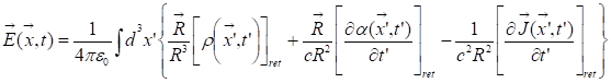 (1)
(1)
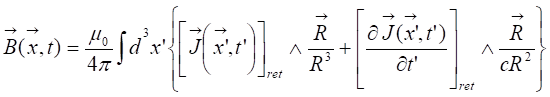 (2)
(2)
where  and
and  are respectively the electric
and magnetic constants, c is the light velocity, a the charge density and
are respectively the electric
and magnetic constants, c is the light velocity, a the charge density and  the
current density. R (
the
current density. R (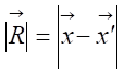 ) is the
distance separating the current sources and observation points while
) is the
distance separating the current sources and observation points while 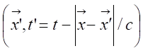 denotes the (retarded)
coordinates of the current source where the electromagnetic waves traveling at
light speed are created.
denotes the (retarded)
coordinates of the current source where the electromagnetic waves traveling at
light speed are created.
The particular case of a ring with a transient current
i is analyzed using the cylindrical coordinates (z,q,r) (see also
the inset of Fig. 1):
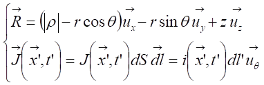 (3)
(3)
where r is the ring radius, S the ring section and dl
the unit length along the ring. As there is no charge density in the ring (a = 0) and
injecting Eq. (3) into Eqs. (1) and (2), the analytical electromagnetic field
in transient regime created by a ring is written in cylindrical coordinates:
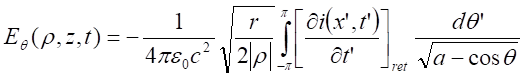 (4)
(4)
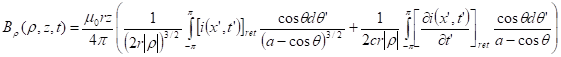 (5)
(5)
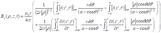 (6)
(6)
with 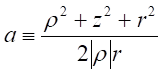
Eqs. (4)-(6) are the generalized equations of Jefimenko for a single
ring with transient current. To confirm the consistence of Eqs. (4)-(6), the
analytical Biot-Savart expression of the magnetic field along the z axis
of the ring with a DC current 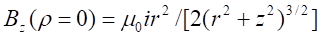 should be
recovered from Eq. (6) by fixing the boundary condition
should be
recovered from Eq. (6) by fixing the boundary condition  and ρ → 0.
The numerical calculations of elliptical functions were done with Mathematica 6.
In Fig. 1, the continuous curve is the magnetic field according to the
analytical equation. The empty circles are the numerical calculated points
using Eq. (6) with
and ρ → 0.
The numerical calculations of elliptical functions were done with Mathematica 6.
In Fig. 1, the continuous curve is the magnetic field according to the
analytical equation. The empty circles are the numerical calculated points
using Eq. (6) with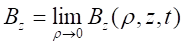 . The good agreement
between the known analytical expression and the calculated one is a validation
of Eq. (6). As an additional check, far from the coil the expression of the
fields should approach those of a radiating magnetic dipole. For that let’s
define the magnetic dipole moment of the ring
. The good agreement
between the known analytical expression and the calculated one is a validation
of Eq. (6). As an additional check, far from the coil the expression of the
fields should approach those of a radiating magnetic dipole. For that let’s
define the magnetic dipole moment of the ring 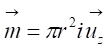 . The static
magnetic dipole assumes a constant current and
a negligible ring radius
. The static
magnetic dipole assumes a constant current and
a negligible ring radius  . With the
later conditions, Eqs. (5) and (6) should be identical with those reported in
literature
. With the
later conditions, Eqs. (5) and (6) should be identical with those reported in
literature 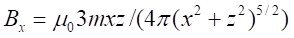 and
and
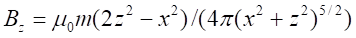 .[xv] Because of cylindrical symmetry, the radial components are equal (
 ). The
magnetic field of a dipole moment is shown in Fig. 2. Four dashed lines are
indexed with letters A, B, C and D. The rescaled magnetic field
). The
magnetic field of a dipole moment is shown in Fig. 2. Four dashed lines are
indexed with letters A, B, C and D. The rescaled magnetic field 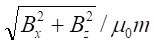 of magnetic
field through these dashed lines are shown in Fig. 3
a) and b) in arbitrary units. Using Mathematica, the Fig. 3
a) and b) show the analytical curves (lines) versus the numerical points
(symbols). The numerical points are obtained with Eqs. (5) and (6) using the
dipole approximations and . The good agreement between
analytical and numerical calculations is a second validation of Eqs. (5) and (6).
Further on, a force study gives the estimation of net thrust between two
coaxial rings.
of magnetic
field through these dashed lines are shown in Fig. 3
a) and b) in arbitrary units. Using Mathematica, the Fig. 3
a) and b) show the analytical curves (lines) versus the numerical points
(symbols). The numerical points are obtained with Eqs. (5) and (6) using the
dipole approximations and . The good agreement between
analytical and numerical calculations is a second validation of Eqs. (5) and (6).
Further on, a force study gives the estimation of net thrust between two
coaxial rings.
III – LOSS OF THE LINEAR MOMENTUM
Assumptions must be given on the dimensionality of the
system. Typical length scales are the size of the emitter and receptor rings,
their separating distance, and the typical wavelength corresponding to the
working frequency. The standard actuators have typically an emitter-to-receptor
distances z around the millimeter, which involves that the
electromagnetic wavelength participating in the force is at maximum in the
order of millimeter. Longer wavelengths cannot excite electrons on the metal
participating in the total force. However, other contribution might come from
the dimension of the system d which is typically at maximum in the order
of decimetre. The frequency  to treat must be higher than the threshold frequency
 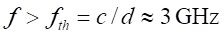 in vacuum.
This relatively high threshold frequency justifies the use of Jefimenko
equations. The Eqs. (4)-(6) take into account the fact that in the transient
regime the waves emitted by different parts of the emitter reach different
parts of the receptor and these in retarded regime, by integrating all the
spatial and temporal effects. However, the calculation of eddy currents is far
from trivial. A deeper Fourier analysis (not shown here) gives the exact
electromagnetic spectrum. The skin depth
in vacuum.
This relatively high threshold frequency justifies the use of Jefimenko
equations. The Eqs. (4)-(6) take into account the fact that in the transient
regime the waves emitted by different parts of the emitter reach different
parts of the receptor and these in retarded regime, by integrating all the
spatial and temporal effects. However, the calculation of eddy currents is far
from trivial. A deeper Fourier analysis (not shown here) gives the exact
electromagnetic spectrum. The skin depth  of eddy currents in transient regime is written as
 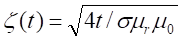 .
. and
and  are the
electronic conductivity and relative magnetic permeability, respectively.[xvi] Note in the transient regime, the skin depth does not
depend on the frequency, but on the time t. A Fourier transform is
therefore useless. Let’s consider thus the interaction between two coaxial
rings, as shown in inset of Fig. 5. The magnetic field B1 is
produced at a time
are the
electronic conductivity and relative magnetic permeability, respectively.[xvi] Note in the transient regime, the skin depth does not
depend on the frequency, but on the time t. A Fourier transform is
therefore useless. Let’s consider thus the interaction between two coaxial
rings, as shown in inset of Fig. 5. The magnetic field B1 is
produced at a time  by means of transient
current
by means of transient
current  . It leaves the emitter ring,
covers the ring-to-ring distance z0 at light speed and starts
inducing the current
. It leaves the emitter ring,
covers the ring-to-ring distance z0 at light speed and starts
inducing the current  in the receptor
ring at a time
in the receptor
ring at a time  . A Laplace force
 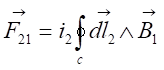 is
created in the receptor ring. The Laplace force is the particular case of
Lorentz force for a current distribution and both are valid in transient
regimes. must be determined from the induced
electromotive force
is
created in the receptor ring. The Laplace force is the particular case of
Lorentz force for a current distribution and both are valid in transient
regimes. must be determined from the induced
electromotive force 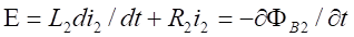 where L2,
R2 and FB2 are respectively the
self-inductance, resistance and magnetic flux of the receptor ring. In the situation
of a transient current pulse
where L2,
R2 and FB2 are respectively the
self-inductance, resistance and magnetic flux of the receptor ring. In the situation
of a transient current pulse 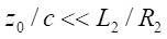 , the
self-inductance term is dominant and the current is simply
, the
self-inductance term is dominant and the current is simply 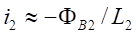 . The field B2,
produced by i2, covers back the ring-to-ring distance and
modifies the current inside the emitter ring at a time
. The field B2,
produced by i2, covers back the ring-to-ring distance and
modifies the current inside the emitter ring at a time 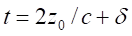 (
( is
a minor delay due to slowing light speed into the metallic crystal of the
receptor ring). Now the emitter ring is subject to the force
is
a minor delay due to slowing light speed into the metallic crystal of the
receptor ring). Now the emitter ring is subject to the force  starting at , and so on. Note that both and
  are times dependent. If the
emitter and receptor rings are jointly attached, the resultant of the system
are times dependent. If the
emitter and receptor rings are jointly attached, the resultant of the system 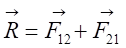 can be calculated in ranges
of times. The normalized instantaneous resultants
can be calculated in ranges
of times. The normalized instantaneous resultants  along
z axis are shown below for the first three ranges of times
along
z axis are shown below for the first three ranges of times  where n indexes the
wave front travel. The initiating transient current starts
at t = 0:
where n indexes the
wave front travel. The initiating transient current starts
at t = 0:
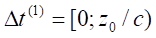
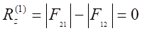 (7)
(7)
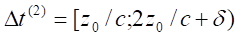
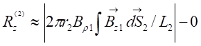 (8)
(8)
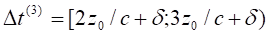
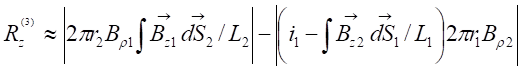 (9)
(9)
where Br1, Bz1, Br2 and Bz2 are calculated using Eqs. (5) and (6).
The induced currents and  decrease versus time and
finally will not significantly contribute to the final force
decrease versus time and
finally will not significantly contribute to the final force  . The maximum
instantaneous resultant is reached in the first receptor-to-emitter
electromagnetic wave travel . After
this range of time, switches simultaneously opening the emitter and receptor
circuits or an adequate signal would reset to zero the currents. Consequently, they
annihilate the Laplace forces F12 and F21. When
after deriving Eqs. (5) and (6), which account all the dynamics of the
electromagnetic field, Eqs. (7)-(9) give the net force versus time and wave
front travel which Eqs. (5) and (6) do not give. To circumvent the space scale
issues, a magnetic core will be introduced in the discussion part.
. The maximum
instantaneous resultant is reached in the first receptor-to-emitter
electromagnetic wave travel . After
this range of time, switches simultaneously opening the emitter and receptor
circuits or an adequate signal would reset to zero the currents. Consequently, they
annihilate the Laplace forces F12 and F21. When
after deriving Eqs. (5) and (6), which account all the dynamics of the
electromagnetic field, Eqs. (7)-(9) give the net force versus time and wave
front travel which Eqs. (5) and (6) do not give. To circumvent the space scale
issues, a magnetic core will be introduced in the discussion part.
Thus, a current pulse into the emitter ring applied
during  and a subsequent opening of
emitter and receptor circuits create a maximum net force
and a subsequent opening of
emitter and receptor circuits create a maximum net force  . The fast opening of circuits
will create a self-induction that will prolong the waiting time by ts-i
before imposing a new pulse into the emitter ring. In short, to continuously
get a net force , a current ramp
should be applied during at a
frequency
. The fast opening of circuits
will create a self-induction that will prolong the waiting time by ts-i
before imposing a new pulse into the emitter ring. In short, to continuously
get a net force , a current ramp
should be applied during at a
frequency  . To get a reasonable thrust
  in vacuum, calculations
showed a working distance and frequency at respectively z0 = 0.1
mm and
in vacuum, calculations
showed a working distance and frequency at respectively z0 = 0.1
mm and  , the latter frequency is out
of current possibilities. The resultant is interesting if only it can be used
not only on time scales of current pulses (typically ns), but on much longer
time scales. The fundamental question is to check the validity of interrupting
the current loops to get a zero force without inducing a counter-induction.
Before having a second current pulse, a subsequent waiting time must get rid of
remaining fields and also of remaining counter-forces. In practice, the ultra
fast current switches can be made using field effect transistors (FETs)[xvii],
ultra fast actuators running at most at 1 GHz[xviii]
or even semiconductor junctions.[xix]
All three should run at very high frequencies.
, the latter frequency is out
of current possibilities. The resultant is interesting if only it can be used
not only on time scales of current pulses (typically ns), but on much longer
time scales. The fundamental question is to check the validity of interrupting
the current loops to get a zero force without inducing a counter-induction.
Before having a second current pulse, a subsequent waiting time must get rid of
remaining fields and also of remaining counter-forces. In practice, the ultra
fast current switches can be made using field effect transistors (FETs)[xvii],
ultra fast actuators running at most at 1 GHz[xviii]
or even semiconductor junctions.[xix]
All three should run at very high frequencies.
Clearly, the inertial, closed and isolated coil-ring
system moves in one direction without applying external forces. The question
raised in the introduction is answered: a thrust is created in the coil-ring
system using retarded fields. An adapted electronics can force the system to
move not only after one current ramp, but also after series of current ramps. A
possible explanation of the observed loss of the mechanical linear momentum is the
loss of the so-called electromagnetic momentum. The electromagnetic waves exert
a pressure, and it is expressed in static regime as follows 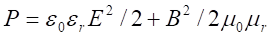 .xiii The total pressure
  present in the coil-ring
system is not symmetric, i.e. the coil exerts an electromagnetic pressure on
the ring placed on only one side of the coil. In the other side of the coil,
the pressure exerted in vacuum is lost and is likely responsible for the
observed loss of the mechanical linear momentum. An additional explanation of
the loss of the momentum is the internal heating. In brief the eddy currents
created in the receptor ring by high frequency electromagnetic waves will be
themselves source of electromagnetic waves. However, the spectrum covered by
these induced waves likely contains infrared light since thermal heating
accompanies eddy currents in metals. To avoid parasitic electromagnetic
crosstalk, a special care must be done on a proper electrical shielding of
current leads.
present in the coil-ring
system is not symmetric, i.e. the coil exerts an electromagnetic pressure on
the ring placed on only one side of the coil. In the other side of the coil,
the pressure exerted in vacuum is lost and is likely responsible for the
observed loss of the mechanical linear momentum. An additional explanation of
the loss of the momentum is the internal heating. In brief the eddy currents
created in the receptor ring by high frequency electromagnetic waves will be
themselves source of electromagnetic waves. However, the spectrum covered by
these induced waves likely contains infrared light since thermal heating
accompanies eddy currents in metals. To avoid parasitic electromagnetic
crosstalk, a special care must be done on a proper electrical shielding of
current leads.
To summarize, the typical working frequencies should
not exceed hundreds of GHz due to the mentioned technical limitations of
switches. The next section discusses a way to reduce the working frequency by
introducing a magnetic core.
IV – DISCUSSION ON A REAL THRUSTER
An option to decrease the frequency in order to have a workable
frequency without losing the amplitude of thrust is
to use a coaxial magnetic guide material with a high magnetic permeability µr
as shown in Fig. 4. The receptor ring is placed in vacuum, in the end of the
core, and therefore its received magnetic field has to be described in vacuum
only. The internal field of the magnetic core will create a phase delay  , discussed in detail below.
At high frequencies the treatment of magnetic field inside a core is simpler
using complex permeability equations than using brutal finite element
calculations such as the Schwarz-Christoffel mapping.[xx] At high frequencies, the magnetic field can be decomposed as
, discussed in detail below.
At high frequencies the treatment of magnetic field inside a core is simpler
using complex permeability equations than using brutal finite element
calculations such as the Schwarz-Christoffel mapping.[xx] At high frequencies, the magnetic field can be decomposed as  in a core and
  in vacuum. The permeability
in transient regime is then deduced as
in vacuum. The permeability
in transient regime is then deduced as 
where  and
and  .[xxi] is an intrinsic value of
magnetic materials and is associated with losses (such as hysteresis or eddy
currents), e.g. in static regime
.[xxi] is an intrinsic value of
magnetic materials and is associated with losses (such as hysteresis or eddy
currents), e.g. in static regime  . An
analytical treatmentxxi gives the loss factor
. An
analytical treatmentxxi gives the loss factor  where
where  and
and  are respectively the
relaxation time of magnetic domains and constant depending on magnetic
susceptibility, under transient magnetic field. While
are respectively the
relaxation time of magnetic domains and constant depending on magnetic
susceptibility, under transient magnetic field. While  increases,
especially for high frequencies, the loss factor
increases,
especially for high frequencies, the loss factor  becomes
small and the remaining losses are attributed by eddy currents losses. They can
be avoided by reducing the dimension of the core in one dimension (hysteresis
losses are also reduced at high frequencies). According to the Fig. 4, the path
followed by the magnetic field suggests that the section at the end of cylinder
can be attributed to a coil without core where the flux FB1 remains the same through the cylinder. As discussed above, the losses
are tiny
becomes
small and the remaining losses are attributed by eddy currents losses. They can
be avoided by reducing the dimension of the core in one dimension (hysteresis
losses are also reduced at high frequencies). According to the Fig. 4, the path
followed by the magnetic field suggests that the section at the end of cylinder
can be attributed to a coil without core where the flux FB1 remains the same through the cylinder. As discussed above, the losses
are tiny  within the range of
frequencies involved (
within the range of
frequencies involved ( ) and such magnetic materials firstly decrease the light speed by a
factor
) and such magnetic materials firstly decrease the light speed by a
factor  and secondly act as a spacer
of length zµr between the two rings. The total distance
separating the two rings is then
and secondly act as a spacer
of length zµr between the two rings. The total distance
separating the two rings is then  where the
receptor ring is placed at z0 from the end of a cylindrical
magnetic core. Then, a current ramp should be applied during
where the
receptor ring is placed at z0 from the end of a cylindrical
magnetic core. Then, a current ramp should be applied during  at frequency
  . Moreover, for a number
  of emitter rings, is proportional to
  and a time delay
  should be taken into account
where
should be taken into account
where  is the spatial elongation of
  wires, see Fig. 4. At
  , were
numerically calculated using Eqs. (5), (6) and (8), e.g. for an emitter ring
radius r1 = 10 cm, a receptor ring inductance L2
= 10 mH, and zµr = 10
cm,
, were
numerically calculated using Eqs. (5), (6) and (8), e.g. for an emitter ring
radius r1 = 10 cm, a receptor ring inductance L2
= 10 mH, and zµr = 10
cm,  mm,
mm,  and
and  (Fig. 5).
  means that the time delay due
to spatial elongation is considered small
compared to the delay of coil-to-ring distance. The current i1
was applied with a ramp of 50 mA/ns. were
calculated versus z0 and for different receptor radius r2.
A maximum force is shown when the two rings have equal radius. When the receptor
ring is near the magnetic core (z0 = 0.1
mm), Fig. 6 shows a maximum of
means that the time delay due
to spatial elongation is considered small
compared to the delay of coil-to-ring distance. The current i1
was applied with a ramp of 50 mA/ns. were
calculated versus z0 and for different receptor radius r2.
A maximum force is shown when the two rings have equal radius. When the receptor
ring is near the magnetic core (z0 = 0.1
mm), Fig. 6 shows a maximum of  for r1
= r2 = 10 cm. The inset of Fig. 6 shows a full period of the
calculated thrust versus time. The
maximum attainable force is
for r1
= r2 = 10 cm. The inset of Fig. 6 shows a full period of the
calculated thrust versus time. The
maximum attainable force is  . The
abrupt force at is due to
. The
abrupt force at is due to  in Eqs. (5) and (6). The low forces in the present thruster with are competitive with other
existing thrusters.i For instance, electrostatic
propulsion system based on Xenon ions reveals a thrust of 0.2 N. Pulsed plasma
using Teflon® shows a thrust of 0.1 N. The main advantage of the
present thruster is the direct conversion of electricity to kinetic energy
without using propellant. There is an way to increase the thrust by increasing . For higher , the delay due to the spatial
elongation cannot be ignored any more.
The force of 130 000 N was reachedii using much higher turns and running a longer time of
current ramp, obtaining then higher magnetic fields. Moreover, the possibility
to play with dimensions, transient currents and magnetic cores help the
experimental feasibility.
in Eqs. (5) and (6). The low forces in the present thruster with are competitive with other
existing thrusters.i For instance, electrostatic
propulsion system based on Xenon ions reveals a thrust of 0.2 N. Pulsed plasma
using Teflon® shows a thrust of 0.1 N. The main advantage of the
present thruster is the direct conversion of electricity to kinetic energy
without using propellant. There is an way to increase the thrust by increasing . For higher , the delay due to the spatial
elongation cannot be ignored any more.
The force of 130 000 N was reachedii using much higher turns and running a longer time of
current ramp, obtaining then higher magnetic fields. Moreover, the possibility
to play with dimensions, transient currents and magnetic cores help the
experimental feasibility.
In conclusion, the generalized equations of Jefimenko
for the single ring with a transient current show good agreement with the
Biot-Savart expression in static regime. A second validation is the good
agreement between analytical and numerical calculations in the dipole moment
approximations. Due to dimensionality, the frequencies f involved in the
resultant force are higher than the threshold frequency 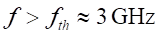 in vacuum.
This relatively high threshold frequency justifies the use of Jefimenko
equations. To circumvent space and time scale issues, a magnetic core is
introduced. The introduction of a magnetic core creates a phase delay that is shown to be small.
The simulations of instantaneous forces between emitter and receptor rings show
the existence of a net thrust in one direction for a small time slot. A direct
consequence is a possible loss of the linear momentum. The thermal heating and
more likely the asymmetrical electromagnetic pressure exerted in the coil-ring
system are responsible for the loss. To benefit of a maximum net
electromagnetic thrust
in vacuum.
This relatively high threshold frequency justifies the use of Jefimenko
equations. To circumvent space and time scale issues, a magnetic core is
introduced. The introduction of a magnetic core creates a phase delay that is shown to be small.
The simulations of instantaneous forces between emitter and receptor rings show
the existence of a net thrust in one direction for a small time slot. A direct
consequence is a possible loss of the linear momentum. The thermal heating and
more likely the asymmetrical electromagnetic pressure exerted in the coil-ring
system are responsible for the loss. To benefit of a maximum net
electromagnetic thrust  , the emitter
circuit should be opened before receiving the magnetic response of the receptor
ring. This latter might be opened at the same time to avoid counter-induction
effects. The experimental requirements are high frequency signals switches into
the emitter and receptor circuits. A thrust of was
obtained for .
, the emitter
circuit should be opened before receiving the magnetic response of the receptor
ring. This latter might be opened at the same time to avoid counter-induction
effects. The experimental requirements are high frequency signals switches into
the emitter and receptor circuits. A thrust of was
obtained for .
ACKNOWLEDGEMENTS
The author would like to thank O.D. Jefimenko for his inspiring
original works.
FIGURE CAPTIONS:
Fig. 1: Continuous line: norm of magnetic field along z axis
according to the known Biot-Savart equation for a ring radius r = 10
cm and a current i = 1 A. Empty circles: norm of magnetic field using
Eq. (6) with the same parameters and with .
The inset shows the ring in the (Oxy) plane, the cylindrical coordinates (z,q,r), the ring radius
r and the observation point.
Fig. 2: Magnetic dipole moment centered at (x;z) = (0;0) using Eqs.
(5) and (6). The four dashed lines are indexed A, B, C and D. See text for more
info.
Fig. 3: Rescaled magnetic field calculated (symbols) with Eqs. (5) and (6) under dipole
approximation versus the rescaled
analytical expressions (dashed lines and lines). The rescaled magnetic fields are
calculated along the x axis a) and z axis b) along two axes
separating the centre (5 and 10 cm).
Fig. 4: Cylindrical magnetic core placed inside the emitter coil.
The receptor ring is placed outside the magnetic core. See text for more info.
Fig. 5: Numerically calculated instantaneous net force (in N) for a system of
emitter-receptor vs. their separating distance z0 and for
different receptor radius r2. The emitter radius was taken r1
= 10 cm, a receptor ring inductance L2 = 10 mH, a magnetic
core with zµr = 10 cm. The current i1 was
applied with a ramp of 50 mA/ns. The inset shows the interaction of two coaxial
emitter (left) and receptor (right) rings. FB1, FB2 are the magnetic fluxes, , the
Laplace force for the receptor and emitter rings respectively. The outer
dashed box represents the system of jointed rings with an instantaneous
resultant . The inset does not show the
magnetic core for simplicity.
Fig. 6: Numerical instantaneous resultant vs. receptors radius r2,
for an emitter-receptor distance z0 = 0.1
mm and an emitter radius r1 = 10
cm. The inset of Fig. 3 shows a full period of the calculated thrust versus time with r1
= r2 = 10 cm, L2 = 10 mH, zµr
= 10 cm and .
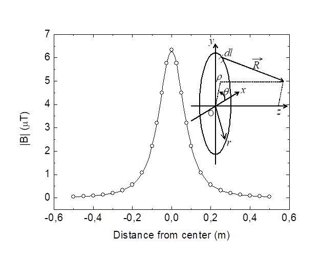
CHARRIER FIG. 1

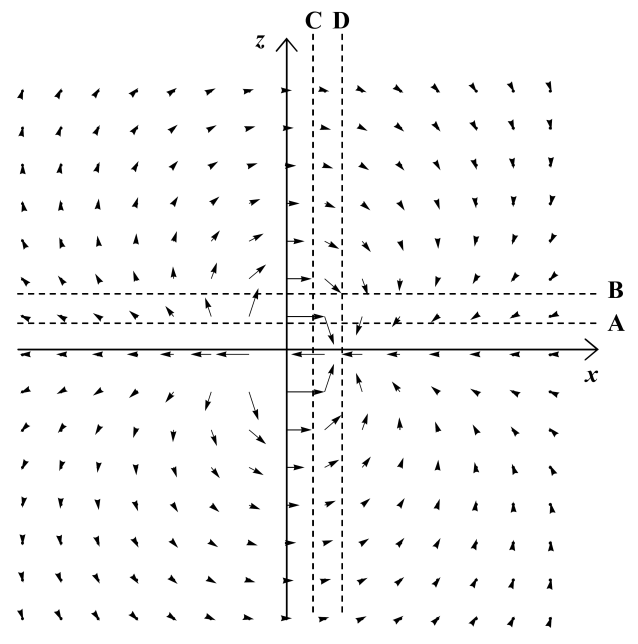
CHARRIER FIG. 2

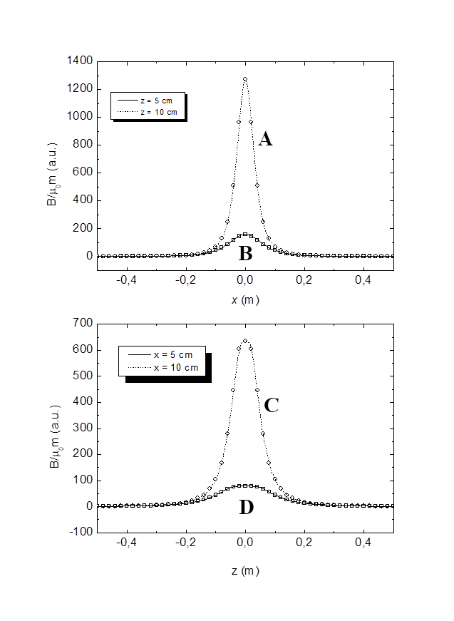
CHARRIER FIG. 3
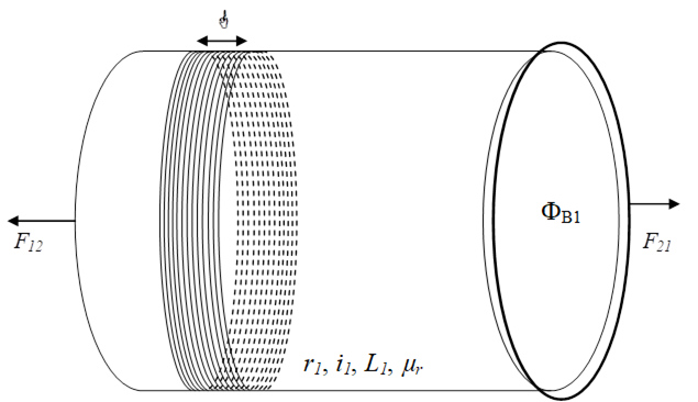
CHARRIER FIG. 4
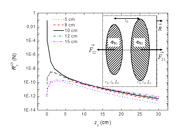
CHARRIER FIG. 5
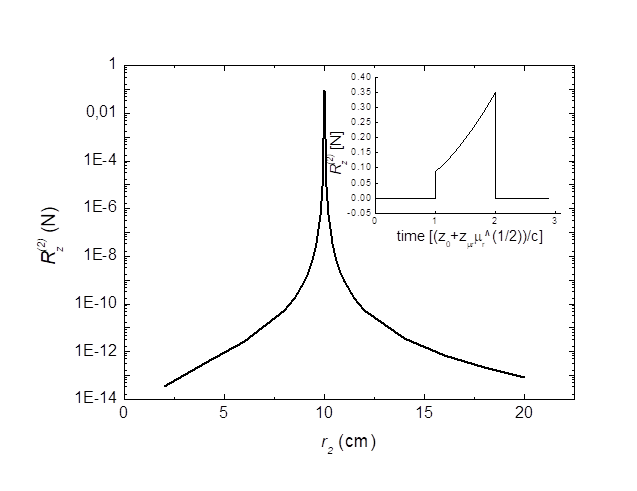
CHARRIER FIG. 6
REFERENCES
Micronewton electromagnetic
thruster
D.S.H.
Charrier
Institut P`
(CNRS – Université de Poitiers – ENSMA), UPR 3346, SP2MI – Téléport 2, Bd Marie
et Pierre Curie, BP 30179, 86962 Futuroscope, France
A low cost and light
electromagnetic thruster, consisting in a disc rigidly attached with a coaxial
coil, shows steady recoil by losing its linear momentum. The signal applied in
the device is a square electric potential. A continuous thrust is observed on
the center-of-mass in one single direction under electromagnetic excitation for
various voltages and nominal high frequencies. At 1 kHz with 20 V amplitude,
the recoil force reaches 4 μN (micronewton). The recoil is numerically
quantified with induced electromotive and Lorentz forces. The presented device
directly converts electric energy into kinetic energy.
Continuous efforts are done for improving performances of thrusters1–8.
Loss of linear momentum between two macroscopic bodies is
demonstrated in the presented device. Classical
electrodynamics is a powerful tool for calculating self-force in current loops9–11
and sometimes leads into linear momentum loss phenomena
between two bodies as soon as retarded interactions play an important role12. It offers a physical way for
producing a thrust, i.e. a direct conversion of electric potential energy into
kinetic energy. This device is hoped to be used in satellites for accurate
trajectory correction maneuvers, for example, thanks to a reduced use of
propellant. The device is designed firstly for creating electromagnetic waves,
secondly for benefiting electrodynamics effects and finally for measuring a
displacement resulting from the lost momentum. The design retained is the
magnetic actuator-like device consisting of a coil and a ring (or a disc). As
for the principle of magnetic actuators13-15, a fast current ramp in
a coil produces a repulsive force in a coaxial metallic ring. Classical magnetic
actuators apply a single ultra fast current ramp (a capacitive discharge) in
order to create, at first wave front travel, a fast magnetic flux variation in
the receptive ring inducing a repulsive Lorentz force. Later, at second wave
front travel, the induced ring has time to create itself a counter force in the
coil and so on, leading to center-of-mass oscillations with damped response.
The counter force, due to the second wave front travel, is supposedly severely
damped because the reemitted electromagnetic field amplitude by the metallic
ring is reduced compared to the emitted one. The amplitude difference is partly
converted into dissipation in the metal. Finally, the total force is due to
asymmetrical properties and geometry between coil and ring. In the device,
series of ultra fast successive current ramps is applied in the coil for
creating a continuous force. The displacement of a rigid coil-disc device is
measured for various voltages and frequencies of excitation. Numerical
calculations of an analytical model partially predict the displacements.
An analytical model of force, after a first wave front travel, was
validated using numerical calculations16. The model recovered both
the Biot-Savard law in the constant uniform current case and the dipole moment
in the dipole approximations. Bρ1 and Bz1
being, respectively, the radial and axial retarded magnetic field components at
the extremity of the coil, they are valid for a small section of coil wire
compared to coil diameter. They are expressed as follows:
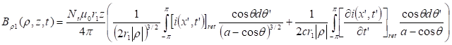 (1)
(1)
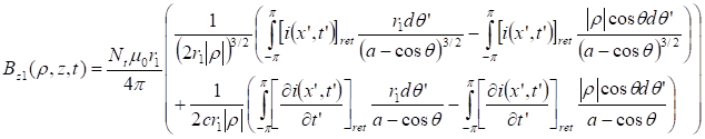 (2)
(2)
with  .
.
 H.m-1 and
  m.s-1 are,
respectively, the magnetic permeability and speed of light in vacuum.
m.s-1 are,
respectively, the magnetic permeability and speed of light in vacuum.  is the time-dependent current
in the coil with retarded coordinates
is the time-dependent current
in the coil with retarded coordinates  .
r1, Nt, r2 and S2
are, respectively, the radius and number of turn of the coil, the radius and
area of the disc. The Lorentz force calculations are chosen instead of those of
Poynting energy flux density because they offer a direct comparison with
experiments. Since the Lorentz force is valid in transient regime, and using
the induced electromotive force, one can deduce the resulting force pushing a
conductive ring with a ultrafast current ramp circulating in a coaxial coil.
The force at first wave front travel is expressed as:
.
r1, Nt, r2 and S2
are, respectively, the radius and number of turn of the coil, the radius and
area of the disc. The Lorentz force calculations are chosen instead of those of
Poynting energy flux density because they offer a direct comparison with
experiments. Since the Lorentz force is valid in transient regime, and using
the induced electromotive force, one can deduce the resulting force pushing a
conductive ring with a ultrafast current ramp circulating in a coaxial coil.
The force at first wave front travel is expressed as:
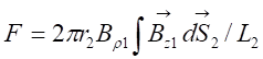 (3)
(3)
where 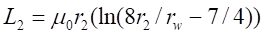 [4] is the inductance of an elementary integration
ring and rw the wire radius of the ring.
[4] is the inductance of an elementary integration
ring and rw the wire radius of the ring.
Here, a disc is used in the experiments instead of a ring because of
higher force sensitivity. The Eq. (3) must integrate the whole disc radius 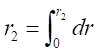 . The wire radius rw
of the ring becomes, by definition, the half thickness of the disc. Finally,
the pushing force on a rigid and coaxial disc is expressed as follows:
. The wire radius rw
of the ring becomes, by definition, the half thickness of the disc. Finally,
the pushing force on a rigid and coaxial disc is expressed as follows:
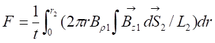 (4)
(4)
where t is the disc thickness. As the coil pushes the disc in
one direction, the idea to glue the disc with the coil as a rigid thruster
leads to consider the force of Eq. (4) as the total force of thruster, at first
wave front travel.
Let’s define, z = zμr + z0
the distance separating the coil and disc. zμr is the distance covered by the magnetic lines in a metallic core before
reaching the vacuum. z0 is the
distance covered by the magnetic lines in vacuum before reaching the disc. In total, the numerical code contains four
physical values (μ0, c, tramp, i1),
six geometrical parameters (r1, Nt, r2,
rw, z0, zμr), three
coordinates of integration (q, r, r). tramp is the ramp duration. In all
calculations presented here, the disc was composed of 100 meshing elements
because a numerical convergence of the force of Eq. (4) was observed between 50
and 1000 meshing elements.
Micro and nanonewton forces can be measured with rotational18,19,
torsion1,20 or translational21 pendulums. As shown in Fig. 1, the rigid coil-disc device was hung on a
translational pendulum by two metallic wires used as current leads at height  of 8.5
cm. The mass pendulum
of 8.5
cm. The mass pendulum  was 76
g. In order to extract torque contributions, two mirrors for displacement
measurements were placed symmetrically with respect to the coil-disc device.
The coil (750 turns Nt) had an interior radius r1
of 8 mm. The core of laminated steel plates was over the coil extremity by a
distance
was 76
g. In order to extract torque contributions, two mirrors for displacement
measurements were placed symmetrically with respect to the coil-disc device.
The coil (750 turns Nt) had an interior radius r1
of 8 mm. The core of laminated steel plates was over the coil extremity by a
distance  of 1.25
cm. The disc (coaxial with the coil and core) with a radius of 1.35
cm for a thickness t (2rw) of 0.6
mm was made of copper. The total distance separating the coil from the disc is
then
of 1.25
cm. The disc (coaxial with the coil and core) with a radius of 1.35
cm for a thickness t (2rw) of 0.6
mm was made of copper. The total distance separating the coil from the disc is
then  +
+  as
mentioned above. The thickness z0 of 0.55
mm was measured optically. A square-shape signal generator (Hameg HM8131-2) was
used as high frequency power supply. The RL frequency fcoil
of the circuit was 476 Hz, while the RL frequency fcoilnocore
without the core was 1380 Hz. The ramp duration tramp
was at nearly 22 ns and the current speed i1 was 14.4
A.ms-1.
as
mentioned above. The thickness z0 of 0.55
mm was measured optically. A square-shape signal generator (Hameg HM8131-2) was
used as high frequency power supply. The RL frequency fcoil
of the circuit was 476 Hz, while the RL frequency fcoilnocore
without the core was 1380 Hz. The ramp duration tramp
was at nearly 22 ns and the current speed i1 was 14.4
A.ms-1.
In Fig. 2 (a), the raw data of displacements versus time measured on
the two channels are shown at rest situation (0 V before 0 second) and with
electromagnetic excitation (100 Hz with amplitude of 20 V after 0 second). The top
and bottom vertical axis are the raw data of measured displacement in
micrometer versus time. Both displacements  and
and
 are positive during
excitation and show a clear deviation from their origin at rest position. The
stronger oscillations appear after the first signal impulses since the most
important kinetic energy is delivered, the coil-disc device going from rest
position to excited position. The device then oscillates around a continuous
displacement until the damping from the pendulum is suppressed. The motion is
created by the continuous electromagnetic excitation and demonstrates a
first-kind electromagnetic thruster. In Fig. 2 (b), successive cycles of
rest/excitation are shown with a periodicity of 200 seconds, the excitation
frequency is 15 MHz at 20 V amplitude. Before 0 second, the device was excited
explaining the damped signal the first hundred seconds. A test situation was to
observe the motion of the coil without copper disc. In the limit of the
experimental accuracy, no displacement was observed agreeing the expectation to
get zero thrust, since no repulsive force was created.
are positive during
excitation and show a clear deviation from their origin at rest position. The
stronger oscillations appear after the first signal impulses since the most
important kinetic energy is delivered, the coil-disc device going from rest
position to excited position. The device then oscillates around a continuous
displacement until the damping from the pendulum is suppressed. The motion is
created by the continuous electromagnetic excitation and demonstrates a
first-kind electromagnetic thruster. In Fig. 2 (b), successive cycles of
rest/excitation are shown with a periodicity of 200 seconds, the excitation
frequency is 15 MHz at 20 V amplitude. Before 0 second, the device was excited
explaining the damped signal the first hundred seconds. A test situation was to
observe the motion of the coil without copper disc. In the limit of the
experimental accuracy, no displacement was observed agreeing the expectation to
get zero thrust, since no repulsive force was created.
In Fig. 3 (a), the real experimental displacement  is shown in μm (Symbols)
versus the voltage amplitude in V at 15 MHz. Numerical calculations of d
(Continuous line) using Eq. (1), (2), (4) and
is shown in μm (Symbols)
versus the voltage amplitude in V at 15 MHz. Numerical calculations of d
(Continuous line) using Eq. (1), (2), (4) and  are shown for comparing the
model and the experiments. Although
the calculated displacement as a function of voltage seems quadratic-like, the
experimental points (without error bars) seem linear. Within
the error bars, the theory fails to explain a weaker experimental displacement
at 20 V. The model can be however used for low voltages. The discrepancy at 20 V between experiment and theory is attributed to less sharp slope of
square excitation signal coming from the power supply, because if less
amplitude of field is delivered into the coil, the total driving force will be
lower as Eq. (4) suggests.
are shown for comparing the
model and the experiments. Although
the calculated displacement as a function of voltage seems quadratic-like, the
experimental points (without error bars) seem linear. Within
the error bars, the theory fails to explain a weaker experimental displacement
at 20 V. The model can be however used for low voltages. The discrepancy at 20 V between experiment and theory is attributed to less sharp slope of
square excitation signal coming from the power supply, because if less
amplitude of field is delivered into the coil, the total driving force will be
lower as Eq. (4) suggests.
In order to see the effect of the excitation frequency on the
displacement, measurements performed with and without steel plates are shown in Fig. 3 (b) on top the top vertical axis. In both cases the
displacement is steady at around 0.5 μm above 1 kHz and the delivered mechanical power in W (bottom
vertical axis) increases. In summary, the low energy consumption of the device
associated with the weak force is very promising for long term applications for
small satellites.
Acknowledgments
The author is very grateful to Fabrice Berneau and Jozef Vesely for
stimulating discussions on the acquisition of data. This work was financially
supported by the French CPER (Région Poitou-Charentes).
Figure captions:
Fig.1: Top view of the device hung on the pendulum. The origin O1
of displacement for mirror 1 is located at rest position of pendulum. The origin
O2 of displacement for mirror 2 is located at rest position of
pendulum.
Fig. 2: Both graphs are measured with a square-shape signal at 20 V
in the coil with core. The top and bottom vertical axis show raw data of
displacement vs. time in micrometer, measured on channel 1 for mirror 1 and on
channel 2 for mirror 2 at 100 Hz (a) and at 15 MHz (b). (b) The signal is
applied with cycled excitations.
Fig. 3: The displacement  is calculated with
  where
and are the displacements
measured on channel 1 and channel 2, respectively. (a) Experimental displacements (Symbols) and
numerical calculations (Continuous line) vs. the excitation voltage at 15 MHz (coil
with core). (b) Experimental displacements and mechanical
power vs. the applied frequency at 20 V.
where
and are the displacements
measured on channel 1 and channel 2, respectively. (a) Experimental displacements (Symbols) and
numerical calculations (Continuous line) vs. the excitation voltage at 15 MHz (coil
with core). (b) Experimental displacements and mechanical
power vs. the applied frequency at 20 V.
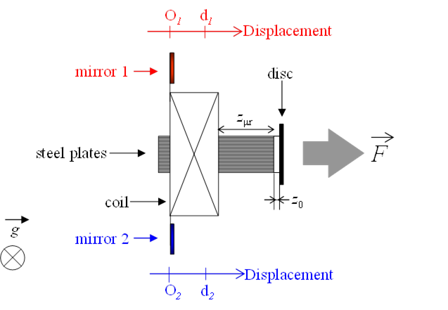
CHARRIER FIG. 1
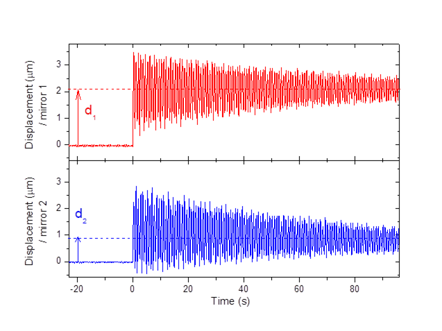
CHARRIER FIG. 2a
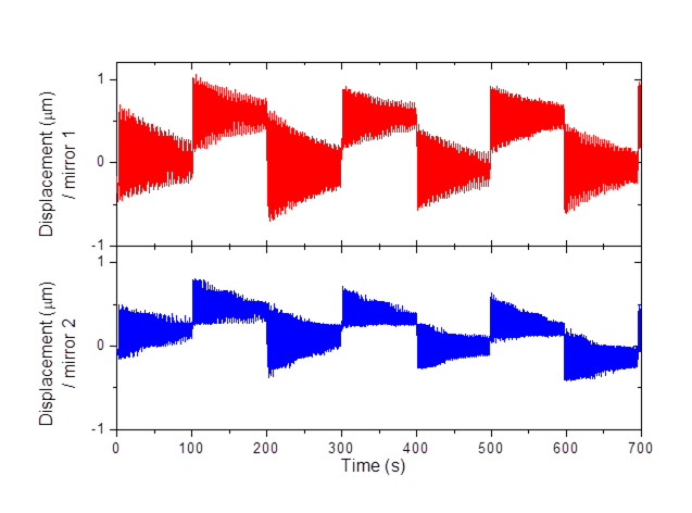
CHARRIER FIG. 2b
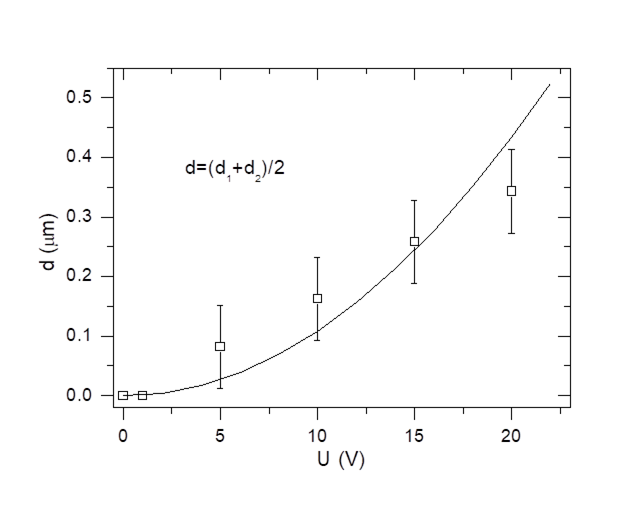
CHARRIER FIG. 3a
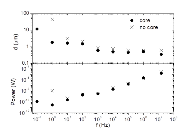
CHARRIER FIG. 3b
References
1 M. Gamero-Castaño, Review of Scientific Instruments 74, 4509
(2003).
2 M. Keidar and I.I. Beilis, Applied Physics Letters 94, 191501
(2009).
3 L. Garrigues, J. Pérez-Luna, J. Lo, G.J.M. Hagelaar, J.P.
Boeuf, and S. Mazouffre, Applied Physics Letters 95, 141501 (2009).
4 F. Taccogna, S. Longo, M. Capitelli, and R. Schneider, Applied
Physics Letters 94, 251502 (2009).
5 M. Martinez-Sanchez and J.E. Pollard, Journal of Propulsion and
Power 14, 688-699 (1998).
6 G. Robertson, P. Murad, and E. Davis, Energy Conversion and
Management 49, 436-452 (2008).
7 T. Yabe, C. Phipps, M. Yamaguchi, R. Nakagawa, K. Aoki, H. Mine, Y.
Ogata, C. Baasandash, M. Nakagawa, E. Fujiwara, K. Yoshida, a. Nishiguchi, and
I. Kajiwara, Applied Physics Letters 80, 4318 (2002).
8 L. Johnson, Review of Scientific Instruments 73, 1079 (2002).
9 G. Ajoy, Physical Review E 74, 067602 (2006).
10 G. Cavalleri, G. Bettoni, E. Tonni, and G. Spavieri, Physical
Review E 58, 2505-2517 (1998).
11 P. Graneau and N. Graneau, Physical Review E 63, 058601 (2001).
12 M.J. Pinheiro, Physica Scripta 84, 055004 (2011).
13 J. Feuchtwanger, E. Asua, A. García-Arribas, V. Etxebarria,
and J.M. Barandiaran, Applied Physics Letters 95, 054102 (2009).
14 L. Straka, N. Lanska, K. Ullakko, and A. Sozinov, Applied Physics
Letters 96, 131903 (2010).
15 B. Kavcic, D. Babic, N. Osterman, B. Podobnik, and I. Poberaj,
Applied Physics Letters 95, 023504 (2009).
16 D.S.H. Charrier, Progress In Electromagnetics Research M 13, 69-82
(2010).
17 J.D. Jackson, Classical Electrodynamics, John Wiley (New York,
1999).
18 V. Nesterov, Measurement Science and Technology 20, 084012 (2009).
19 A.N. Grubišić and S.B. Gabriel, Measurement Science and
Technology 21, 105101 (2010).
20 S.K. Lamoreaux, Physical Review Letters 78, 5-8 (1997).
21 S. Rocca, C. Menon, and D. Nicolini, Measurement Science and
Technology 17, 711-718 (2006).
This article was prepared in response to reactions of the 2012
paper. It was a complementary communication with the conference held in
Baltimore in the American Physical Society.
Frequency spectrum analysis on the force contribution in a micronewton
electromagnetic thruster
D.S.H.
Charrier,†
*Institut P` (CNRS – Université de Poitiers – ENSMA), UPR 3346, SP2MI – Téléport 2,
Bd Marie et Pierre Curie, BP 30179, 86962 Futuroscope, France
†Nexans Research Center, 29 rue Pré
Gaudry, 69007 Lyon, France
A frequency analysis on results published in 2012 is given in this
letter, where experimental displacements of the coil-disc device obtained at
different generator square signal frequencies (from 100 Hz to 15 MHz) are
compared with monochromatic AC currents calculated from RL and RLCstray
circuit impedances. In time domain, a square signal can be decomposed in sum of
monochromatic (Dirac-like) contributions in frequency domain. The analysis
revealed that i) the RL circuit has a working device onset frequency above 170
kHz ii) the stray capacitance Cstray of the coil must be much below
the order of pF for having working coil-disc device frequencies. The onset
frequency at 170 kHz is coherent with a previous prediction, the device having
decimeter scale d at maximum, the monochromatic working threshold frequency was
found at about fth = c/d » 3 GHz.
In 2012, experimental results were reported on an electromagnetic
thruster1 although a similar original concept was reported before by
Goodwin.2,3 Since then, the order of magnitude of thrust or at least
the proof-of-principle on a laboratory scale device were not reported by other
works. The thrust was explained by an electromagnetic momentum emitted by the
coil transferred into mechanical momentum on the metallic disc. Transient
regime, asymmetrical coil-disc device, Joule heating accompanying eddy currents
helped in creating a total net force and not only on short time scales. In this
letter, different physical and theoretical aspects are given to complement past
experiments that could help experimentalists willing to reproduce the
proof-of-principle and a frequency signal analysis is reported. The force
equation was proposed and confronted to experimental results with a relative
success:
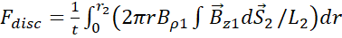 Equation 1
where t, r2, r, Br1, Bz1, S2 and L2 are respectively, the disc thickness, the disc and integration
radius, the radial and axial magnetic field components at the extremity of the
coil, the disc area and the ring integration inductance. Experiments were
performed with an angle between the geological north-sourth line and the coil
axis at 15°. The disc was oriented to the south-east and the coil to the
north-west. Measurements were performed at Latitude: 46.66 and Longitude: 0.36.
A magnetic field component (along Bz1) such as the Earth magnetic
field which is not time dependent within the time scale of experiments does not
create a force on the disc since only the time dependent fields contribute into
the force of Equation 1. The issue of surrounding environment of the coil-disc
system contributing to the total thrust might be raised when taking into
account sources of artifacts, such as mirror charging effects. A care was taken
in order to prevent proximity mirror effects by using an immediate environment
made of wood.
Recently,
works were published on either advices4 or recommendations5
for measuring respectively micronewton or even nanonewton. In Ref1,
optical fibers placed in the vicinity of a metal plate collected reflected
light. It was shown that the reflected light is linearly proportional to the
fiber to metal plate distance in a certain range of distance.6 The
link between collected light and displacement was done using a calibration
curve: input reflected light voltage versus displacement in micrometer measured
with a micrometer screw. Regarding the acquisition of displacements, the
following procedure was followed: acquisition at rest position, a pause of
acquisition just before switching on the power supply, few seconds of waiting
time, acquisition again. The few seconds of waiting time of displacement
acquisition was necessary due to the too high displacement provoked by the
first square shape ramps up of the signal. This minor note about the transient
regime does not change the displacement observed in the steady regime which was
used for the analysis. Therefore all the data as shown in 1 do not
show few seconds of displacement after the power supply was switched on.
Moreover, complementary trials were performed where the two optical fiber
sensors were placed in opposite direction in such way that all artifacts
between the coil-disc device and the measurement setup was uncorrelated.
Regarding the model and the interpretation of the results, several comments are
given here. As proposed by Lafleur7, the need to consider the speed
of sound is of interest when looking at the force establishment on the whole
body. The calculations proposed in here8 were to consider the total
force at a time t without regarding any mechanical steady state or relativistic
effect. Since the total motion of the rigid or elastic body under non-uniform
acceleration is also source of intense investigations, as referenced by
Franklin9 and Dmitriev10, no further model was built. As
shown in Table 1, the measurement setup and the device characteristics can be
decomposed in different frequency spectrum. The terms ‘monochromatic’ and
‘polychromatic’ refer respectively to Dirac-like frequency and rich Fourier
decomposed frequency spectrum. The thrust measurement setup was composed by
pendulum and sampling frequencies. Both are monochromatic. The oscillating
frequency of the pendulum 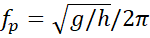 = 1,71 Hz
with g the standard
gravitational constant (9,81 m s-2) and h the pendulum height (8,5 cm) is crucial
when working a low generator square wave frequency. To be relevant, the generator
frequency must be at least two times higher than the pendulum oscillating
frequency. At low frequency the system coil hung on the pendulum might enter
into resonant oscillations. The sampling frequency
= 1,71 Hz
with g the standard
gravitational constant (9,81 m s-2) and h the pendulum height (8,5 cm) is crucial
when working a low generator square wave frequency. To be relevant, the generator
frequency must be at least two times higher than the pendulum oscillating
frequency. At low frequency the system coil hung on the pendulum might enter
into resonant oscillations. The sampling frequency  was about 10
Hz. The data of displacements done with a generator frequency above
was about 10
Hz. The data of displacements done with a generator frequency above  = 20 Hz were relevant. As shown in Table 1, the coil was excited
with a square wave generator where the periodic wave is monochromatic and the
Fourier decomposed square signal is necessary polychromatic. From the disc
side, both working device electromagnetic wave frequencies and eddy current and
skin depth frequencies are polychromatic.
= 20 Hz were relevant. As shown in Table 1, the coil was excited
with a square wave generator where the periodic wave is monochromatic and the
Fourier decomposed square signal is necessary polychromatic. From the disc
side, both working device electromagnetic wave frequencies and eddy current and
skin depth frequencies are polychromatic.
In order to identify the unknown working frequency of the device,
complementary calculations in frequency domain are presented. The calculations
presented in Ref 1 used a linear and resistive ramp up to calculate
the current and its derivative as function of time. Here the RL circuit is
treated rather than simple resistive R circuit. Then the Equation 2 was used to
calculate the current.
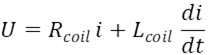 Equation 2
where U, i, Rcoil and Lcoil are respectively the
voltage, current, resistance and inductance of the coil. Taking conditions of icoil(t=0) = 0 and t = Lcircuit/Rcircuit then both current
and its derivative can be calculated as a function of time as shown in Equation
3, Equation 4 and in Figure 1.
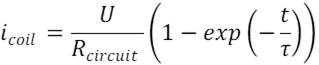 Equation 3
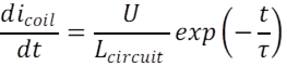 Equation 4
In frequency
domain, the RL circuit is described using the impedance terms as shown in
Equation 5:
 Equation 5
where w is equal et 2pf with the f
the frequency of the signal. Using the norm of impedance, it is possible to use
the impedance to deduce the current flowing in the coil in one single
frequency,
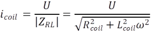 Equation 6
Using the frequency domain, the derivative
dicoil(w)/dt is equal at zero.
Inductances are
known to behave as capacitor at high frequencies because the presence of
isolated spires influence themselves. As shown in Figure 2, the stray
capacitance coming from the inductance is added in the impedance calculations.
The impedance term is shown in Equation 7.
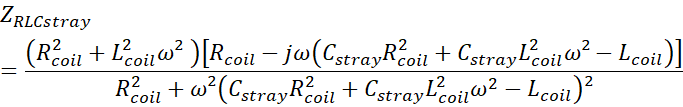
Equation 7
where Cstray is the stray
capacitance that is to be defined. Impedance terms contrarily to Equation 3 and
Equation 4 allow a frequency-domain study rather than a time-domain study. As
shown in Figure 3, according to the stray capacitance values (RLC
circuit), the current in the coil has a minimum while in the case of RL circuit
the current decreases with the frequency. In Figure 4, the experimental and
calculated displacements are shown. The experimental displacement was obtained
with the so-called polychromatic square wave generator while the calculated
displacements are monochromatic coming from the impedance terms. The aim of
this representation is to identify the working monochromatic frequencies. For
instance, in the case of stray capacitance of value 1 pF, less than two decades
of frequencies are involved in the displacement while in the case of RL or RLC
with 1 fF, a large working frequency spectrum is identified above 170 kHz
(~1,8
km wavelength). Electromagnetic momentum transfer into mechanical momentum in
the disc is possible using a continuum spectrum of Dirac-like frequencies above
170 kHz. Indeed frequencies below 170 kHz are not playing a role in the force.
This observation is consistent with what it has been proposed in the past8.
In term of experimental improvements, the exciting signal must be monitored
accurately in order to extract the full Fourier decomposed spectrum. The same
spectrum can be inserted in the calculation and confronted to experiments. The
force can be increased by decreasing the resistivity of disc, using low
temperatures. Stray capacitance can be reduced by replacing N spires into a
single large flat metal sheet or using electronic means of compensation.
Figure captions:
Figure 1: Current
i and its derivative di/dt in time domain in the RL device circuit.
Figure 2:
Equivalent circuit of the operational device under electromagnetic excitation.
Stray capacitance between the coil spires changes the device response.
Figure 3:
Currents calculations in monochromatic frequency domain using RL and RLC
impedances (1 nF and 1 pF stray capacitances).
Figure 4: Real
displacement as produced by a polychromatic square wave generator (Fourier
decomposition of a square contains infinity a monochromatic frequencies) versus
monochromatic calculated displacements.
Tables:
Table 1:
Decomposition of frequencies present in the experiments reported in Ref1.
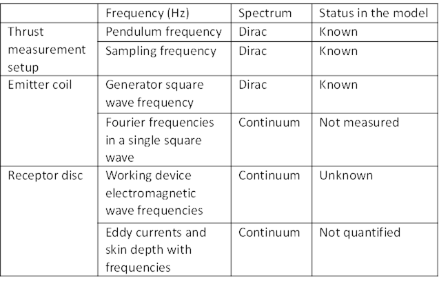
CHARRIER TABLE1
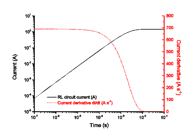
CHARRIER FIG. 1
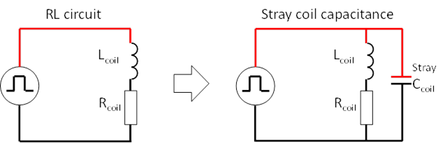
CHARRIER FIG. 2
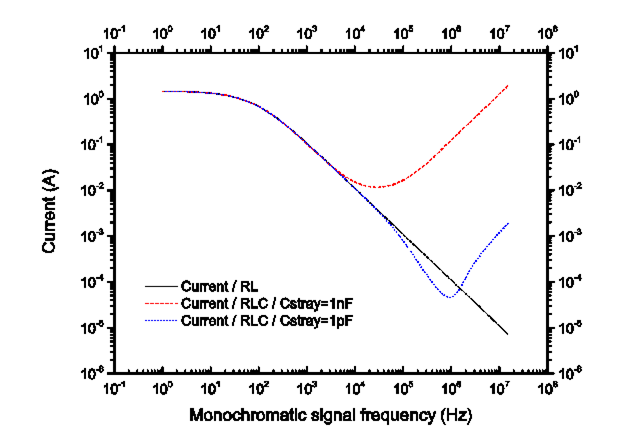
CHARRIER FIG. 3
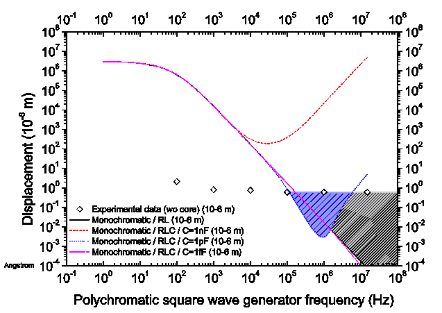
CHARRIER FIG. 4
References
1 D.S.H. Charrier, Appl. Phys. Lett. 101, 034104 (2012).
2 D.P. Goodwin, AIP Conf. Proc. 552, 976 (2001).
3 D.P. Goodwin, AIP Conf. Proc. 699, 1175 (2004).
4 J. Soni and S. Roy, Rev. Sci. Instrum. 84, 095103 (2013).
5 J.E. Polk, A. Pancotti, T. Haag, S. King, M. Walker, J. Blakely,
and J. Ziemer, in 33rd Int. Electr. Propuls. Conf. (2013), pp. 1–24.
6 C. Coupeau, J.C. Girard, and J. Grilhé, J. Vac. Sci. Technol. B
Microelectron. Nanom. Struct. 16, 1964 (1998).
7 T. Lafleur, Appl. Phys. Lett. 105, 146101 (2014).
8 D.S.H. Charrier, Prog. Electromagn. Res. M 13, 69 (2010).
9 J. Franklin, Found. Phys. 43, 1489 (2013).
10 A.L. Dmitriev, AIP Conf. Proc. 969, 1163 (2008).
|
|
Name
|
SI unit
|
Symbol
|
Symbolic expression
|
|
Mass
|
kilogram
|
M
|
kg
|
|
Length
|
meter
|
L
|
m
|
|
Time
|
second
|
T
|
s
|
|
Current
|
ampere
|
I
|
A
|
|
|
Temperature
|
kelvin
|
T
|
K
|
|
|
Volt
|
volt
|
U
|
kg.m2.s-3.A-1
|
|
|
Resistance
|
ohm
|
Ω
|
kg.m2.s-3.A-2
|
|
|
Inductance
|
henry
|
H
|
kg.m2.s-2.A-2
|
|
|
Capacitance
|
farad
|
F
|
kg−1.m−2.s4.A2
|
|
|
Electric field
|
|
|
kg⋅m⋅s−3⋅A−1
|
|
Chap. 1
|
Force
|
newton
|
N
|
kg.m.s-2
|
|
Work, Energy, Heat
|
joule
|
J
|
kg.m2.s-2
|
|
Power
|
watt
|
W
|
kg.m2.s-3
|
|
Chap.
2
|
Momentum
|
|
|
kg.m.s-1
|
|
Magnetic induction
|
tesla
|
T
|
kg.s-2.A-1
|
|
Pressure
|
pascal
|
Pa
|
kg.m-1.s-2
|
|
Term
|
Definition extracted from en.oxforddictionaries.com
|
|
Truth
|
That which is true or in
accordance with fact or reality.
|
|
Proof
|
Evidence or argument
establishing a fact or the truth of a statement.
|
|
Effect
|
A physical phenomenon,
typically named after its discoverer.
|
|
Phenomenon
|
A fact or situation that is
observed to exist or happen, especially one whose cause or explanation is in
question.
|
|
Law
|
A statement of fact,
deduced from observation, to the effect that a particular natural or
scientific phenomenon always occurs if certain conditions are present.
|
|
A generalization based on a
fact or event perceived to be recurrent.
|
|
Theorem
|
A general proposition not
self-evident but proved by a chain of reasoning; a truth established by means
of accepted truths.
|
|
Lemma
|
A subsidiary or
intermediate theorem in an argument or proof.
|
|
Principle
|
A fundamental truth or proposition
that serves as the foundation for a system of belief or behavior or for a
chain of reasoning.
|
|
A general scientific
theorem or law that has numerous special applications across a wide field.
|
|
Postulate
|
A thing suggested or
assumed as true as the basis for reasoning, discussion, or belief.
|
|
Axiom
|
A statement or proposition
which is regarded as being established, accepted, or self-evidently true.
|
|
Hypothesis
|
A supposition or proposed
explanation made on the basis of limited evidence as a starting point for
further investigation.
|
|
A proposition made as a
basis for reasoning, without any assumption of its truth.
|
|
Scepticism
|
A sceptical attitude; doubt
as to the truth of something.
|
|
Criticism
|
The expression of
disapproval of someone or something on the basis of perceived faults or
mistakes.
|
|
Constant in physics
|
|
Value
|
Unit
|
|
Speed of light in vacuum
|
c
|
299 792 458
|
m.s-1
|
|
Boltzmann constant
|
k
|
1.38064852 × 10⁻²³
|
kg.m2.s-2.K-1
|
|
Newtonian constant of
gravitation
|
G
|
6.67408(31) × 10-11
|
kg−1⋅m3.s−2
|
|
Planck constant
|
h
|
6.626 070 040(81) × 10-34
|
kg.m2.s-1
|
|
Magnetic constant
|
µ0
|
4p × 10-7
|
kg.m.s-2.A-2
|
|
Electric constant
|
e0
|
8.854 187 817 × 10-12
|
kg−1.m−3.s4⋅A2
|
|
Electric charge
|
C
|
1.602 × 10⁻¹⁹
|
s.A
|
|
Stefan-Boltzmann constant
|
s
|
5.670 367 × 10-8
|
kg.s3.K-4
|
Figure 1‑1 The author performing the
air flux trap with a ping pong ball
Figure 1‑2 Potential energy
distribution of ultrasonic standing wave [15]
Figure 1‑3 “Kugel fontain”: a stone
levitating with a film of water [14]
Figure 1‑4 Ti Zr-Ni alloy in an
electrostatic levitator chamber (Physics Today)
Figure 1‑5 Are room temperature
superconductors possible? [26]
Figure 1‑6 Iron ball floating in air [20]
Figure 1‑7 Instable potential well
(saddle like) under static magnetic field
Figure 1‑8 The author performing a
diamagnetic levitation of a B pencil lead
Figure 1‑9 Free fall axis
Figure 1‑10 Apparent and pseudo-stable
levitation
Figure 1‑11 Stable levitation model
Figure 2‑1 Permanent magnet creates a
force F in a conductor with a current I
Figure 2‑2 Cylindrical coil
represented with magnetic flux lines
Figure 2‑3 Conical coil represented
with magnetic flux lines
Figure 2‑4 Schematic of two masses
Figure 2‑5 Circle on which mass the M
stays confined in closed circuit
Figure 3‑1 Definitions of (1) open,
(2) closed, and (3) isolated systems
Figure 3‑2 Coil-ring device with
magnetic field lines
Figure 3‑3 Assumption of a disc as
being discretized with multi-rings
Table 1‑1 Newton's laws of motion [1],
[2]
Table 1‑2 Einstein’s
postulates of special relativity [3]
Table 1‑3
Consequences of special relativity
Table 1‑4 Laws of electromagnetism [4]
Table 1‑5 Laws of thermodynamics
Table 1‑6 Thermal
radiation laws
Table 1‑7 Ways for
levitating solid objects met in Nature and technologies
Table 1‑8 Complete
map of magnetic levitation and examples
Table 1‑9 Magnetic
susceptibilities of different elements [30]
Table 3‑1
Qualitative assessment of different cases where heat dissipation and work are
confronted in the device coil-disc
I give the reasons why I chose the quotes
for each chapter.
Page 1:
I first read this quote in 1998 at
the library of the Jopeph Fourier University. It summarizes the notion of
‘concrete’ as being the ‘abstract’ becoming familiar by use. Let’s say that
life, laws of Nature are irrational. Even if equations can describe the
dynamics of motions and interactions, in particular we do not know the origin
at physical constants.
Page 24:
First quote
If our eyes could only see perfectly
symmetrical systems, or only equilibrium situations, we would not be able to
catch unexpected phenomena and consequently not able to anticipate any new experiments.
I think creativity must born from asymmetry in Nature, also of course from
provoked situations.
Second quote:
In my opinion, any question must be
animated by a fast or a long process of search. To give an answer to all
questions is not mandatory while the approach of constant questioning is. The
process of (fast or long) searching is healthy, a constant questioning too.
Page 34:
First quote
This quote is very important. In
other words, the rational point of view must invite anyone to separate the
person bringing a message from the content of the message. Personally I prefer
to discuss on the content of a message rather on its author. Seriousness of a
messenger can sometimes bring seriousness in his message, this is rarely
reciprocal, i.e. a message from an author with a poor fame will not have a same
impact than a famous one.
Second quote
Indeed a hard work defeats
everything. Here, the work is not quantifiable in Joule. Also, a lot of work
and energy can defeat gravity.
[i] M. Tajmar, Advanced Space Propulsion Systems (Springer-Verlag,
Wien New York, 2002).
[ii] P. B. Zieve, J. L. Hartmann, and J. K. Ng, IEEE Transactions on
Magnetics 24, 3144 (1988).
[iii] O. D. Jefimenko, Causality, Electromagnetic Induction and Gravitation
(Electret-Scientific-Company, West Virginia, 2000).
[iv] O. D. Jefimenko, Electricity and Magnetism (Appleton-Century
Crofts, New York, 1966).
[v] J. J. Monaghan, J. Phys. A 1, 112 (1968).
[vi] C. Mayes and G. Hoffstaetter, Phys. Rev. ST Accel. Beams 12,
024401 (2009).
[vii] A. O. Barut, Phys. Rev. D 10, 3335 (1974).
[viii] C. Teitelboim, D. Villarroel, and Ch. G. van Weert, Rivista Del
Nuovo Cimento 3, 1 (1980).
[ix] D. Villarroel, Phys. Rev. E 66, 046624 (2002).
[x] J. A. Heras, Am. J. Phys. 62, 1109 (1994).
[xi]
J. A. Heras, Phys. Rev. E 58, 5047 (1998).
[xii]
J. L. Jiménez, I. Campos, and N. Aquino, Eur. J. Phys. 29, 163 (2008).
[xiii] J. D. Jackson, Classical Electrodynamics (John Wiley &
Sons, New York, 1999).
[xiv] D. J. Griffiths and M. A. Heald, Am. J. Phys. 59, 111 (1990).
[xv] E. M. Purcell, Electricity and Magnetism Berkeley Physics Course
Volume 2 (McGraw-Hill, New York, 1985).
[xvi] A. Krawczyk and J. A. Tegopoulos, Numerical Modelling of Eddy
Currents (Oxford University Press, New York, 1993).
[xvii] S. R. Weinzierl and J. P. Krusius, IEEE Trans. Electron devices 39,
1050 (1992).
[xviii] K. L. Ekinci and M. L. Roukes, Rev. Sci. Instrum. 76, 061101
(2005).
[xix] S. K. Lyubutin, S. N. Rukin, B. G. Slovikovsky, and S. N. Tsyranov,
Tech. Phys. Lett. 31, 36 (2005).
[xx] M. Markovic, M. Jufer, and Y. Perriard, IEEE Transactions on
Magnetics 44, 2181 (2008).
[xxi] M. Getzlaff, Fundamentals of Magnetism (Springer-Verlag, Berlin
and Heidelberg, 2008).